Haskell Types
by Carl Burch, Hendrix College, August 2012
Haskell Types by Carl Burch is licensed under a Creative Commons Attribution-Share Alike 3.0 United States License.
Based on a work at www.cburch.com/books/hstype/.
Contents
2. Classes
3. Enumerated types
4. Types with nested data
5. Parameterized types
1. Polymorphic functions
In our function types thus far, we've worked with specific
types. But Haskell also has a feature where functions can work
with arbitrary types.
Recall, for example, our threshold function.
threshold :: Double -> (Double -> Double) -> (Double -> Double)

threshold z f = g where g x = min z (f x)
We've written the type for threshold so that the
function only works for functions from Doubles to
Doubles. But we can be more lenient:
threshold would work just as well
on functions from Integers to Doubles, or for
functions from Strings to Doubles.
Enter polymorphic functions, where we can have type “variables” (there's that nasty word again) that represent an abstract type to based on how the function is actually used. In Haskell, each type variable is generally a lower-case letter.
threshold :: Double -> (Double -> a) -> (Double -> a)In this case, we're saying to let a be the type of the first parameter function's parameter; the returned function's parameter must also be of that type.
The composition function (.) is an interesting case to
study with polymorphic types.
Recall that we defined it as the following.
f . g = h where h x = f (g x) -- as defined in the PreludeNow what's the most general type we could assign to this function?
We'll start with x, the parameter to h, the return
value, and assign it a type variable a.
Notice that x is passed to g also, so g must also take a
parameter of type a.
Let's suppose that g returns a value of type b
(which may or may not be the same as a).
To compute h, the return value of f is passed into f, so
f's parameter type must be b.
Whatever f returns — call it c — is likewise
returned by h. This leads to the following type declaration.
(.) :: (b -> c) -> (a -> b) -> (a -> c)2. Classes
Below is a definition of the built-in function min. What
type should it have?
min x y = if x < y then x else yThe simple thing to do would be to define min to
simply take two Doubles as parameters and return a
Double. But declaring it that way means that we can't
use min to work on integers or strings — though it
seems quite reasonable that it should work on integers and
strings. We'd like a more generic type for this function.
We can see that x, y, and the return value must all
be of the same type, which suggests “a -> a -> a” as
min's type. But this is too broad: We have to be able to use the
less-than operation on x and y. We need some way
to be able to constrain a to be a type that supports
less-than comparisons.
Haskell has an answer for that, called classes, where we can say that a type belongs to a class (is a class instance) since it includes functions that the class requires. Despite the usage of the word class and instance, this has nothing to do with object-oriented programming; a Haskell class is closer to a Java interface.
In this case, we want the built-in class named Ord.
To be an instance of that class, a type must include the
comparison operators
<,
>,
<=,
>=,
==, and
/=. The built-in types Integer and Double
are instances of the Ord class (as is String).
The following type signature indicates that min's type
uses a type variable a that must represent an instance
of Ord:
min :: Ord a => a -> a -> aWe can similarly use Ord to give threshold
additional flexibility, so that it can work with functions whose
return values are strings or integers, in addition to functions
whose return values are Doubles.
threshold :: Ord a => a -> (b -> a) -> (b -> a)3. Enumerated types
We can also define new types beyond those built into Haskell. For example, suppose that we want to have a type for playing cards. We first want to declare a data type for card suits, which we can accomplish as follows.
data Suit = Clubs | Diamonds | Hearts | SpadesIn this case, we've declared that Suit is a new type
with four possible values.
We could very reasonably wish to ensure that this new Suit
type is an instance of some class.
For example, if we want to allow the equality operator ==
to apply to Suits, we might write the following.
instance Eq Suit where

    Clubs    == Clubs    = True

    Diamonds == Diamonds = True

    Hearts   == Hearts   = True

    Spades   == Spades   = True

    x        == y        = False
The first line here says that we're trying to justify that
Suit is part of the Eq class, a built-in class
that includes == and /=. (We saw Ord
earlier: It extends Eq by adding the comparison operators
<, <=, > and >= ?.)
Following the where, we need to define the ==
operator as it applies to Suit.
In this case, we define == by first listing the cases
where they are equal, and then by listing a catch-all case so
that any other combination is treated as unequal.
The Eq class also requires the /= operator.
However, it also defines that if /= is not defined for a type,
then it can be derived from the definition of ==.
So we can safely omit it, and /= will automatically be
defined for Suit based on our definition of ==.
Our definition of Suit's == function does
look rather repetitive. In fact, Haskell provides a shortcut
for types that simply enumerate the possible values, including
Suit: When we define the type, we use the deriving keyword
to indicate that a default implementation should be defined.
data Suit = Clubs | Diamonds | Hearts | Spades deriving (Eq, Show)Here, we've said that our new Suit type should be given
a simplistic definition of Eq and Show. The
default definition for Eq is what we have already seen.
We haven't seen the Show class, but it requires the
definition of the show function that maps values of the
class to strings. Because Suit now is an instance of Show,
we can give a Suit value to the show function to
get its corresponding string: “show Hearts”
yields the string “Hearts”.
Note that deriving can only be used for
data types that are defined by listing the individual values to
be used. In the remainder of this document, we'll define some
other data types (Card and BinTree) that are
more flexible, and we cannot use deriving for them.
4. Types with nested data
Now that Suit is defined, we can go on to define the
type for an individual playing card. One way we could do this
would be to simply list all the possible values
(AceOfSpades, TwoOfClubs, et cetera),
but that's unwieldy. Instead, we'll build up the type using
other types at our disposal.
data Card = Joker | Ranked Integer SuitWe've listed Joker as one particular value that
Card can have. But we've also listed Ranked,
which is essentially a two-parameter function that creates a
Card value. In a program, I could write
“Ranked 2 Clubs” to represent the two of
clubs.
To define a function involving cards, we will typically use pattern-matching both to address possible cases and to retrieve any data nested in the value.
isFaceCard :: Card -> Bool

isFaceCard Joker        = False

isFaceCard (Ranked r s) = r > 10
We can similarly use this pattern-matching technique to indicate that we should be able to test whether two cards are equal.
instance Eq Card where

    Joker      == Joker        = True

    Ranked r s == Ranked r' s' = r == r' && s == s'

    Joker      == Ranked r s   = False

    Ranked r s == Joker        = False
We haven't seen strings yet, but we'll soon see that we can
use double-quotes to talk about a string constant and ++
to catenate two strings together. Using this, we can define
Card as an instance of Show as well.
instance Show Card where

    show Joker = "Joker"

    show (Ranked r s) = (show r) ++ " of " ++ (show s)
5. Parameterized types
When we define a data type, we're also allowed to include a variable that represents some other type. (This is akin to a generic class in Java or template in C++.) For example, we would want to define a binary tree so that the type of value stored in each node can be customized.
data BinTree a = Empty | Node a (BinTree a) (BinTree a)With this in hand, we can now work with a BinTree Integer,
or a BinTree String, or even a BinTree Card.
Note that in any of these cases, it is a recursive type:
A Node has not only a value but also two more
BinTree's within it (but of the same types as the overall
tree.
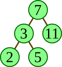
The following illustrates how one can creating a particular binary tree (namely, the one illustrated at right).
ps = Node 7

       (Node 3 (Node 2 Empty Empty) (Node 5 Empty Empty))

       (Node 11 Empty Empty)
One function we might want to define on this is a function to compute the height of a tree. In this case, we don't care about the individual values stored in the tree at all.
depth :: BinTree a -> Integer

depth Empty = 0

depth (Node _ left right) = 1 + max (depth left) (depth right)
A more involved function would be to use this for a binary
search tree, and then to define a function to determine whether
a value exists in the tree. We'll need the values to have the
various comparison operators associated with it, so we'll need
to require that the values within each node have a type that
conforms to the Ord class.
contains :: Ord a => a -> BinTree a -> Bool

contains x Empty = False

contains x (Node val left right) = if x == val then True

                                   else if x < val then contains x left

                                   else contains x right
Now let's define BinTree to be an instance of the
Eq class. Doing this will involve testing that the value
within each corresponding node is equal, so we will need the
values' type itself to be an instance of the Eq class.
We'd wrie this constraint into the first line as follows.
instance Eq a => Eq (BinTree a) where

    Empty == Empty = True

    (Node v lft rt) == (Node v' lft' rt') = v == v' && lft == lft' && rt == rt'
Similarly, we can define BinTree to be an instance of
Show, but we'll need a way to convert each individual
value within each node into a string — so the type of the
node's values would need to be an instance of sh Show ? as
well.
instance (Show a) => Show (BinTree a) where

    show Empty = "()"

    show (Node val Empty Empty) = "(" ++ (show val) ++ ")"

    show (Node val left right) = "(" ++ (show val) ++ " " ++

                                 (show left) ++ " " ++ (show right) ++ ")"
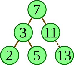
Finally, let's define an insert function that adds a
value into a binary search tree. In an imperative language, we'd
do this by altering a single pointer at the bottom of the tree
to point to a new node (figure (a) below).
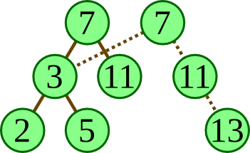
Of course, this isn't possible in a functional
language, since it involves changing the state of the tree.
But we can simply “rebuild” the nodes along the path
to where the value should be inserted (figure (b) below).
|
|
| (a) imperative insert | (a) functional insert |
The following function definition implements this rebuilding process to construct a new root with the value inserted.
insert :: Ord a => a -> BinTree a -> BinTree a

insert x Empty = Node x Empty Empty

insert x (Node val left right) = if x < val

                                 then Node val (insert x left) right

                                 else Node val left (insert x right)