Chapter 1. Introduction
In this book, our goal is to understand
computation. In particular, we want to be able to take any
computational problem and produce a technique for solving it that is
both correct and efficient.
1.1. Procedure and data
Computation is built of two basic elements: procedure and
data. (See Figure 1.1.) This fact is
succinctly summarized by the title of a 1970s computer science textbook,
Data Structures + Algorithms =
Programs (by Niklaus Wirth, from Prentice Hall, 1976).
This binary nature is reflected in object-oriented languages
such as Java: Here, each object has two major categories of
components, instance methods (i.e., procedures) and
instance variables (i.e., data).
Figure 1.1: The two sides of the computation coin.
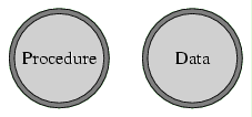
Like energy and mass are physical phenomena
united by Einstein's formula
E = m c²,
procedure and data are
to some extent two different ways of viewing the same thing.
Computer users understand this intuitively: While we often
talk about a program being a procedure, in fact a program is text
representing the procedure, and that text is just a long string
of characters — that is, data. The compiled program, too, is simply a file on
disk containing data. We understand this intuitively today, but
understanding programs as just another form of data was a
breakthrough in the early hisory of computing:
In the ENIAC, introduced in
1946 as the first American computer, each task required
rewiring the hardware, until in 1948, when the ENIAC was wired
to be able to read programs as data from its own memory. This concept,
called the von Neumann computer, quickly caught on. (In
the reverse direction, Alonzo Church developed the
theory of lambda calculus in the 1930s to study
the fundamentals of computing. In his system, each integer and
indeed every other piece of data is represented as a procedure.)
Any computational problem will involve both data and procedure
in its solution. Sometimes the data portion or the procedure
portion will be simple; but it is still present. Take, for
example, the computational problem of determining whether
a number is prime. Before we can begin a procedure for
determining this, we must first have
the number in question, which after all is data.
The representation of this data is simple but important.
You might assume that the number would arrive us in its Arabic
representation
(e.g., 1003). But the problem is somewhat different if it comes in
Roman representation (MIII) or Chinese representation
( ).
).
In fact, the representation of data can dramatically affect the
efficiency of a procedure. Suppose, for example, if instead of
an Arabic representation, the number is instead given us in terms
of its prime factorization (17 ⋅ 59). Then the procedure
will be much more efficient: We simply to check whether the prime
factorization contains more than one number.
This theme of how data should be represented will form a major
portion of this book. We won't spend too much time on
simple data like numbers, though:
Our focus will be on representing a large collection of data so that
it can be processed efficiently. Such techniques for storing data
collections are called data structures, and we'll see
several throughout the book.
1.1.1. Abstract data types
But before we get to data structures, we first need the concept
of an abstract data type (often abbreviated ADT), which
refers to a particular set of operations we want to be able to
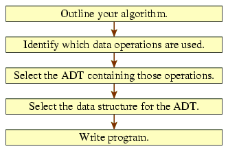
perform on a collection. Given an algorithm to solve a problem
using a collection of data, we should be able to identify which
operations are necessary on that collection, and then we find
the ADT that matches it. Once we know which ADT to use, we can then
select the appropriate data structure based on others' work
concerning how best to implement the ADT.
This program design process is summarized by the following
diagram.
Figure 1.2: The steps to developing a data-intensive program.
In this book, we'll examine several ADTs and the data structures
commonly used for them. One ADT is
the Set ADT, intended for algorithms that use
a data collection like a mathematical set. Operations in the
Set ADT include:
size to get the number of elements in the
set.
contains(x) to test whether a particular element
x lies within the set.
add(x) to insert an element x into the
set, returning true if x is newly added. (As a
set, we wouldn't add x if it were already present.)
remove(x) to remove an element x from the
set.
This ADT is quite useful;
our study of it will be deferred, though, to
Chapter 5.
Another ADT that we'll study is the List ADT, where elements are
stored in a particular order. The List ADT contains the
following operations.
size to get the number of elements in the list.
add(x) to add a value x to the end
of a list.
get(i) to fetch the element at index
i of the list.
set(i, x) to change the element at index
i of the list to be x instead.
add(i, x) to insert an element x
into the list at index i.
remove(i) to remove an element at index
i from the list.
Although the List and Set ADTs are similar, they have some
important differences. With the List ADT, each element is
considered to be at
a particular index, whereas the Set ADT
has no notion of ordering; on the other hand, the Set ADT
includes a contains operation that is absent from the
List ADT.
In the course of this book, we'll study both of these ADTs
along with others that people have found useful over the years.
Our primary emphasis, though, will be on the best data
structures to use for implementing them.
This understanding enables writing efficient
algorithms for many important problems. We'll study a sampling
of these problems in the course of this book.
1.1.2. Interfaces
You might notice that the ADT concept resembles Java's concept
of interface: Both are abstract sets of operations.
The concepts are not entirely equivalent, though.
One difference is that the
ADT concept is intended to be language-neutral; the language
doesn't need a construct similar to Java interfaces for the
ADT concept to be useful. Another difference is
that ADTs are really meant only for large masses of
data, whereas Java programs use interfaces for other
purposes, too.
If we're programming in Java, though, it's easy enough to define
an ADT in terms of an interface.
public interface Set<E> {

    public int size();

    public boolean contains(E value);

    public boolean add(E value);

    public E remove(E value);

}
public interface List<E> {

    public int size();

    public boolean add(E value);

    public E get(int index);

    public E set(int index, E value);

    public void add(int index, E value);

    public E remove(int index);

}
Indeed, these interfaces are already built into Java's
java.util package — but they include many more methods beyond
those listed above, too.
(In this book, we'll study many of the interfaces and
classes defined in the java.util package.
Figure 1.3 lists all of those we'll study.)
Figure 1.3: Parts of the java.util package appearing in this
book.
| Interfaces | Classes |
|---|
| List | ArrayList |
| Set | LinkedList |
| Iterator | TreeSet |
| ListIterator | TreeMap |
| Map | HashSet |
| HashMap |
Perhaps you have not before seen the <E> notation used above.
These definitions use
a feature of Java called generics, where we can designate
an identifier — E in this case — to represent an
arbitrary class; that is, the identifier acts something like a
variable that stands for a type.
When we use the interface, we'll specify what class the
variable E should be taken to stand for. For List and
Set, the individual elements of the collection will be instances
of this class. (In fact,
the E stands for element.) As an example of using these
generics, if we want to declare a variable names to represent
a list of strings, we could write the following.
List<String> names;
We can later create a List of Strings and assign names
to refer to it.
Then, names's get method will
return a String, since, after all, the get method's
return type is E, and in names's case,
E refers to the String type.
String first = names.get(0);
If the notion of generics is unfamiliar to you, then you should
read a Java book and become familiar with the
concept. (Generics were introduced with Java 5; you won't
find much information about the concepts in books preceding its
release date of Summer 2004. Previous to Java 5,
the java.util classes worked with Objects.)
Before continuing, note quickly that the Set and List
interfaces contain several methods in common.
The interface designers carefully named them the same so that
programmers could remember them more easily.
One peculiar thing about the commonality is the
add method. In the Set interface, the method returns a
boolean, so that it can indicate whether the value
needed to be added to the set. (A set doesn't include any
elements twice.) Just to be consistent, the designers made List's
add method return a boolean also, but
in fact add's return value will always be true
with a List.
To use the List interface, we need some way of getting at
List objects. Of course, since List is an interface, we can't
write new List
to create List objects in a program. We can
only create List objects through creating instances of an
implementation of the List interface. We'll see one such
implementation next: the ArrayList class. In the next chapter,
we'll see another implementation, the LinkedList class.
1.2. The ArrayList data structure
The array is the fundamental data structure built into Java
for holding collections of items. Arrays provide
two basic operations: You can retrieve the value at an
index, or you can change the value at an
index. These are quite similar to the List ADT's
get and set operations.
| array operation | equivalent List ADT operation |
|---|
x = data[i]; |
x = get(i) |
data[i] = x; |
set(i, x) |
This similarity is what inspires the implementation of the List
interface using an array to store the data elements.
There are other List operations
that don't correspond to anything we can do
with an array (add and
remove); but this is a detail that we can hope to
overcome.
Overall, it seems like an array is a good candidate for
implementing the List interface.
Java's built-in libraries already include such an implementation;
specifically, the java.util package includes the ArrayList class.
To use it, you need to include a import statement at
the top of your program definition.
import java.util.ArrayList;
Like the List interface, the ArrayList class is a generic.
Inside a method definition, we can declare a names
variable and then assign it to refer to a newly created
ArrayList object.
List<String> names;

names = new ArrayList<String>();
Once we have a way of referring to an ArrayList object,
then we can tell it to do things using the ArrayList methods,
which necessarily include all the methods in the List interface.
Among these is the add method.
names.add("Martin");

names.add("Galloway");
Suppose we want to display all the strings in the ArrayList.
List's size and get methods are useful for
this.
for(int i = 0; i < names.size(); i++) {

    System.out.println(names.get(i));

}
1.2.1. Relationship to arrays
It's important to remember that despite the name, arrays are completely
unrelated to ArrayLists. (Ok, there is something of a relationship: The
programmers who wrote the ArrayList class implemented it using arrays.
But this is private information in the class, and normal
programmers don't ever look inside the ArrayList implementation,
so this relationship doesn't have any direct impact when programming.)
This lack of relationship means that you can't confuse the
syntax for accessing them.
If you have an ArrayList names, you cannot use
the subscripts used with arrays, as in names[0] = "Harpo";
; instead, you
must use the more cumbersome notation names.set(0, "Harpo");
.
An ArrayList, after all, is a regular object, and thus the only
operation you can perform on it is to access its public methods
(and public variables, if it had any).
Similarly, if data is a String[] variable — that is,
an array of Strings —, you cannot write
data.add("Harpo");
to grow the array.
An array's size is fixed at the time of the array's creation.
When we're programming, how should we decide between using an
array and an ArrayList?
While arrays are more convenient for accessing
elements by index, that convenience comes at the price of
missing the List methods (particularly the automatic-growth
behavior of add).
The fundamental question to ask, then, is whether you are
confident that
the array's size will not change once the collection is created.
If so, then you should choose to use an array.
But if the structure might need to adapt its size,
you should choose an ArrayList; you won't get to use the special
array syntax for accessing elements, but the automatic growth
will make up for it.
ArrayLists offer one other advantage over arrays:
They have some additional methods that we haven't covered that
can be useful. The most notable is the indexOf
method, which takes an element as a parameter and returns the
index at which that element first occurs in the list — or, if
it doesn't occur at all, −1.
Even if you have a fixed-length structure, then, the ArrayList
may still be a better choice.
1.2.2. Wrapper classes
A significant limitation of ArrayLists (and List and Set
implementations generally) is that they can contain only
objects. This isn't usually much of a limitation, since
virtually every data item in Java is an object. But Java
includes a few types that aren't classes (i.e., the type of an object).
These are called primitive types, and Java includes
eight, including int,
boolean, and double. (The other five are
char, byte, short, long,
and float.) Java distinguishes the
primitive types from the object types by using names
starting with lower-case letters, while classes' names are
conventionally capitalized.
So we can't put an int into an ArrayList. But what if
we want a list of integers? For cases like this, Java provides a
wrapper class for each of the eight primitive types;
each instance of the wrapper class is an object with a single
instance variable, whose type is the corresponding primitive type.
The wrapper class for int is named
Integer. While ArrayList<int>
is illegal
because int is not a class, Integer is a class, and so
ArrayList<Integer>
is fine.
ArrayList<Integer> primes = new ArrayList<Integer>();
We can now add Integers into the list. But remember that an
int is not an Integer, so we cannot write
primes.add(2);
.
Fortunately, we can easily create an
Integer object wrapped around an int.
primes.add(new Integer(2));

Java (since Java 5) has a
feature called autoboxing, where the compiler will
automatically convert between Integers and ints
when necessary. Thus, we actually can write
primes.add(2);
. The compiler will notice the
bug
and silently translate it to
primes.add(new Integer(2));
.
Similarly, the compiler will add a call to intValue
were we to write primes.get(0) + 1
.
Sounds nice, no? But it has some major problems. One such is
that == and != work
differently for objects, so that primes.get(0) == 2
is false, whereas
primes.get(0).intValue() == 2
is true.
(In fact, the situation is even more complex: The first example would
be true on some computers and false on others.)
For this, and for other reasons,
I advise against using autoboxing, and this book will not make
use of it.
Integer objects are not eligible for mathematical operations like
addition. Thus, when we extract an Integer from the ArrayList, we will
probably want to get the int value it is wrapped around. The
Integer class's intValue method returns this int.
int three = primes.get(0).intValue() + 1;
As you can see, having to use Integers rather than int is
a bit of a pain — but with practice, the pain isn't really
much of a problem.
There are no methods in the Integer class for altering the value
inside the wrapper object. If you want a wrapper object for a
different value, you must create a wholly new instance of the
wrapper class.
1.2.3. Using ArrayList
As an example of a problem where the List ADT is useful,
consider the problem of finding the number of primes up to and
potentially including n.
Mathematicians call this function π(n); for example,
π(11) is 5 because four primes (2, 3, 5, 7, 11) are at most
11.
I realize that it's a stretch to think of a scenario where somebody's
livelihood depends on this quantity, but still it's an
interesting problem.
Incidentally, mathematicians have proven that π(n)
is approximately n / ln n.
Figure 1.4 tabulates a few values of
π(n)
(computed using our program) to check how close this approximation
is.
Figure 1.4: A sampling of values for π(n).
| n |
π(n) |
n / ln n |
error |
| 100 | 25 | 21.7 | 13.1% |
| 1,000 | 168 | 144.8 | 13.4% |
| 10,000 | 1,229 | 1,085.7 | 11.7% |
| 100,000 | 9,592 | 8,685.9 | 9.4% |
| 1,000,000 | 78,498 | 72,382.4 | 7.8% |
| 10,000,000 | 664,579 | 620,420.7 | 6.6% |
You can see that the error appears to be slowly converging to 0.
The mathematical proof, though, is more difficult:
Legendre conjectured the formula in 1798, and it was proven
nearly a century later in 1896, independently by Hadamard and
de la Vallée Poussin.
The algorithm we'll use, implemented in
Figure 1.5, involves creating a collection of
all the primes up to n. (We'll see later, in
Section 4.1, that this isn't the most efficient
algorithm.)
We'll start with the collection containing
just the number 2, and then we'll iterate through the odd numbers
up to n. For each odd number k, we'll determine whether it belongs
in the collection by seeing whether any of the primes already
present divide into k.
Figure 1.5: Counting primes using the ArrayList class.
// Returns the number of primes that are <= n.

public static int countPrimesTo(int n) {

    List<Integer> primes = new ArrayList<Integer>(n);

    primes.add(new Integer(2));

    for(int k = 3; k <= n; k += 2) {

        if(testPrimality(k, primes)) primes.add(new Integer(k));

    }

    return primes.size();

}


// Tests whether k is prime using the primes listed.

private static boolean testPrimality(int k, List<Integer> primes) {

    for(int i = 0; true; i++) {

        int p = primes.get(i).intValue();

        if(p * p > k) return true;   // we passed sqrt(k); k is prime

        if(k % p == 0) return false; // we found a divisor; k is not prime

    }

}
The algorithm used in Figure 1.5 has a small
bug. Do you see it? It illustrates a common programming problem:
Whenever you write a program, you should thank about how it
works for the extreme cases. Frequently, a program that works
for most cases will fail on the easiest cases. In this case, the
program works wrongly when n is given as 1: It will report
that there is a prime less than or equal to 1, when in fact the
first prime is 2. This bug is easy to fix: We can just add an
if statement as the first line saying to return 0
if n is less than 2.
The implementation takes advantage of a simple but major
efficiency help: In testing whether a number k is
prime, we need only check for factors up to sqrt(k). After
all, if k has a factor above sqrt(k) —
call it p — then k / p would also be a factor, and k / p
would be less than sqrt(k) since
p > sqrt(k).
Thus, if k has any factors,
some of them must be less than or equal to sqrt(k).
Initially, the Set ADT may seem a more appropriate choice for
representing the collection of primes, since the index of each
individual prime doesn't matter. But for the efficiency
improvement to take hold, we would like to be able to go through the
collection in ascending order so that we can stop once we
reach sqrt(k). (Also, checking smaller
primes first is a good idea because these are
more likely
to divide large numbers.)
The List ADT allows us to keep the primes in order as we would
like.
1.2.4. Implementing the ArrayList class
Programmers can theoretically use ArrayLists without really
understanding how they work: After all, Java developers have already
built the class into the java.util package. Good
programmers, though,
need to understand the class's internals in order to understand the
performance of ArrayList's methods.
Figure 1.6 contains a possible way of writing the
ArrayList class so that it implements all of the List methods we
discussed earlier.
Figure 1.6: An ArrayList implementation.
  1  public class ArrayList<E> implements List<E> {

  2      private E[] elements; // values stored in current list

  3      private int curSize;  // number of element in current list

  4

  5      public ArrayList(int capacity) {

  6          elements = (E[]) new Object[capacity]; // ignore this

  7          curSize = 0;

  8      }

  9

 14      public int size() {

 15          return curSize;

 16      }

 17

 18      public E get(int index) {

 19          return elements[index];

 20      }

 21

 22      public E set(int index, E value) {

 23          E old = elements[index];

 24          elements[index] = value;

 25          return old; // should return previous value at index

 26      }

 27

 28      public boolean add(E value) {

 29          // see text about handling case when array is full

 31          elements[curSize] = value;

 32          curSize++;

 33          return true;

 34      }

 35

 48      public void add(int index, E value) {

 49          // see text about handling case when array is full

 51          for(int i = curSize - 1; i >= index; i--) {

 52              elements[i + 1] = elements[i];

 53          }

 54          elements[index] = value;

 55          curSize++;

 56      }

 57

 58      public E remove(int index) {

 59          E old = elements[index];

 60          for(int i = index + 1; i < curSize; i++) {

 61              elements[i - 1] = elements[i];

 62          }

 63          curSize--;

 64          return old; // should return previous value at index

 65      }

 70  }
(The ignore this
comment of
line 6 refers to the peculiar
technique that appears for creating an array of generic objects. We
want to say
elements = new E[capacity]
, but Java doesn't handle
this relatively obscure construct properly. Thus,
line 6 must work around Java's
limitation. If the workaround doesn't
make sense to you, don't worry about it.)
As you can see, it involves two instance
variables: elements, an array containing all
of the list's current values, and curSize, the
number of elements currently in the list.
Conceptually, the ArrayList starts out empty, but it will grow
through calls to the add method.
Behind the scenes, though, invisible to programmers using
the class, the array is created once when the object is created,
and rather than grow,
the class simply uses more of the
array that was created at the outset.
The size and get methods are straightforward;
the set
method is only slightly more complicated because the List
interface specification requires that the method
return the value previous to the requested change at that index.
The remove method is complicated by the need to shift
all of the elements forward in the array over the removed item.
The implementation in Figure 1.6 has an
important limitation: We can only add as many elements as we
specify at the time we construct the array. The array can't
grow
after being created in line 6
— and, indeed, Java arrays have no way of growing
once they are created.
The ArrayList class built into the java.util package gets around
this by instead using an add method similar to that of
Figure 1.7.
Figure 1.7: Modifying add to extend array when full.
public boolean add(E value) {

    ensureElements(curSize + 1);

    elements[curSize] = value;

    curSize++;

    return true;

}


// Ensures that elements array has the desired length by

// creating a longer copy if necessary.

private void ensureElements(int desired) {

    if(elements.length < desired) {

        E[] newElements = (E[]) new Object[2 * elements.length];

        for(int i = 0; i < elements.length; i++) {

            newElements[i] = elements[i];

        }

        elements = newElements;

    }

}
With this method, once the
current array becomes filled, it switches to a new, longer array,
being careful to copy the old values into the new
array. As the programmer, you don't need to worry about when
this happens: It all happens behind the scenes, transparently.
This process of creating a new array and copying all of
the old values takes a lot of time,
but this happens quite rarely —
and, if we double the length of the array each time, it becomes
increasingly rare as the array becomes longer.
Overall, then, it doesn't really affect performance
dramatically.
The ArrayList class also includes a constructor including no
arguments, which starts the capacity out at a small value (10).
public ArrayList() {

    this(10); // enters the other constructor, giving capacity of 10

}
Using this constructor, the programmer doesn't have to guess the list's
initial capacity. Instead, using the amended add
method, the program will simply grow the array to be large
enough to fit the actual data.
