Prefix notation is also sometimes called
Chapter 5. Trees
In Chapter 2, we studied one form of recursive data
structure, where each node (a ListNode object) has a single
reference to another node.
In this chapter, we'll study the obvious extension:
What if each node has references to two other next
nodes?
We'll get a diagram like the following.
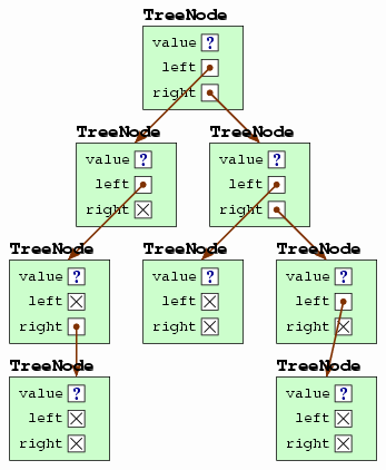
We call such a structure a tree. It may strike you as a peculiar name for such a structure; the name derives from the fact that if you turn the page upside down and squint really hard, the diagram looks vaguely like a bush. (Try it.)
5.1. Fundamentals
Before looking at how trees are used for implementing ADTs, we'll begin with some fundamental concepts, including basic tree terms, memory representation, simple theory about tree quantities, and a specific application of trees to representing mathematical expressions.
5.1.1. Terminology
Computer scientists talk about trees a lot, and consequently they have a large set of terminology to refer to different pieces of the tree. Luckily, the terminology is mostly intuitive, although the mixed metaphors are sometimes a bit confusing.
Technically, a
Neither, incidentally, is a doubly linked list a tree, because each node in the middle of such a list is referenced twice — once by its preceding node and once by its succeeding node. A singly linked list, however, is a tree, though it's a degenerate one.
The following diagram illustrates some of the important terms for a tree.
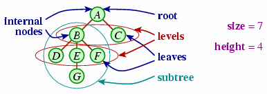
The node at the tree's top (A in the diagram) is called
the tree's
The terminology for talking about relationships between nodes
derives from thinking of the tree as a diagram of a person's
descendants. We would say that B and C are
A
We'll sometimes talk about the
We will sometimes quantify
characteristics of a tree.
The most basic measure of a tree is its
5.1.2. Tree data structures
To represent a single node in a binary tree, we will use the TreeNode class of Figure 5.1.
Figure 5.1: The TreeNode class.
  1  class TreeNode<E> {

  2      private E value;

  3      private TreeNode<E> left;

  4      private TreeNode<E> right;

  5

  6      public TreeNode(E v, TreeNode<E> l, TreeNode<E> r) {

  7          value = v; left = l; right = r;

  8      }

  9

 10      public E           getValue()       { return value; }

 11      public TreeNode<E> getLeft()        { return left; }

 12      public TreeNode<E> getRight()       { return right; }

 13

 14      public void setValue(E v)           { value = v; }

 15      public void setLeft(TreeNode<E> l)  { left = l; }

 16      public void setRight(TreeNode<E> r) { right = r; }

 17  }
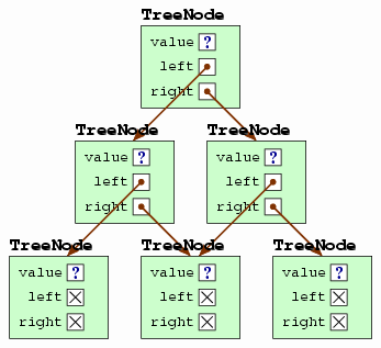
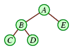
Each TreeNode stores three pieces of data: the node's value, the node's left child, and the node's right child. The following illustrates the creation of a tree structure using this class, with the tree diagrammed at right.
TreeNode<String> root =

    new TreeNode<String>("A",

        new TreeNode<String>("B",

            new TreeNode<String>("C", null, null),

            new TreeNode<String>("D", null, null)),

        new TreeNode<String>("E", null, null));
With this TreeNode class defined, we can define methods that work with the tree. Since a tree is a recursive structure, the most convenient way to write many such methods is via recursive calls. The following is an example of such a recursive function; it computes a binary tree's size (the number of nodes).
public static int countNodes(TreeNode root) {

    if(root == null) return 0;

    else return 1 + countNodes(root.getLeft()) + countNodes(root.getRight());

}
Another example is the following method to compute a tree's height.
public static int height(TreeNode root) {

    if(root == null) return 0;

    else return 1 + Math.max(height(root.getLeft()), height(root.getRight()));

}
If you imagine the recursion tree for either these methods, you should see that it essentially traces the tree being processed.
5.1.3. Relating tree quantities
We have seen two basic measures of a tree: its size and its height. It's natural for us to ask how they are related. In particular, suppose we have a binary tree of size n. What does this tell us about its height?
One easy thing to say about the tree's height is that it can be no larger than n. This comes from considering a tree where each node has one child except for the last. (This amounts to a singly linked list.) We can also say something about the minimum height: The smallest possible height is 2 — the root on one level, and its n − 1 children on the other.
But with a binary tree, the analysis of the minimum height is
somewhat more complicated. To do this, we'll first define the
term
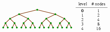
Let us define Mh to be the size of the complete binary tree with height h. We can tabulate the first few values of Mh to get a feeling for how it works.
| h | Mh |
|---|---|
| 1 | 1 |
| 2 | 3 |
| 3 | 7 |
| 4 | 15 |
Based on this, you might suppose that Mh = 2h − 1. But we'll prove it.
We'll first prove that in a complete tree, each level has twice as many nodes as the previous level. Thus, we assert, level k of a complete binary tree has 2k nodes (numbering our levels starting at 0): We can convince ourselves of this by observing that it is true for k = 0 — the root level — where there is just 1 = 20 node. And then we observe that if level k − 1 has 2k − 1 nodes, then level k will have 2 ⋅ 2k − 1 = 2k nodes, since each node in level k − 1 has exactly two children in level k.
This technique of argument, called an induction proof, is particularly convenient when talking about data structures: An induction proof starts by establishing that the assertion is true for a starting case (the base case), and then proving the induction step — that if the assertion holds starting with the base case and going up to k − 1, then the assertion would also hold for k. With both steps completed, then we can conclude that it holds for all integers beyond the base case.
We'll use another induction proof to prove that Mh = 2h − 1. First the base case: Note that M1 is 1, which is indeed 21 − 1. Now, for the induction step: Suppose that we already knew that Mh − 1 = 2h − 1 − 1. The last level of the height-h complete tree is level h − 1, which we just showed contains 2h − 1 nodes. Thus, Mh will be 2h − 1 more than Mh − 1, and starting from here and simplifying we can conclude that Mh is 2h − 1, as we want for the induction step:
| Mh | = | Mh − 1 + 2h − 1 |
| = | (2h − 1 − 1) + 2h − 1 | |
| = | (2h − 1 + 2h − 1) − 1 | |
| = | 2 ⋅ 2h − 1 − 1 | |
| = | 2h − 1 |
This completes the induction proof.
Since Mh = 2h − 1 is the maximum number of nodes in a binary tree with height h, it must be that for any tree, 2h − 1 is greater than or equal to n, where h is the height of that tree and n is the number of nodes in that tree:
We'll solve for n:
h ≥ log2 (n + 1)
This says that a binary tree with n nodes has a height of at least log2 (n + 1).
5.1.4. Expression trees and traversals
Trees pop up quite frequently in computer science. We've already seen one instance in recursion trees — though in that case it was not a data structure but a technique for diagramming computation.
Another place where trees naturally arise is in representing arithmetic
expressions using an
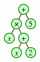
Figure 5.2 contains five classes that demonstrate how we could represent an expression tree in Java. As you can see, it includes an abstract class and four concrete subclasses.
Figure 5.2: Classes for representing an expression tree.
public abstract class Expr {

    public abstract int eval(int value);

}
public class AddExpr extends Expr {

    private Expr left;

    private Expr right;


    public AddExpr(Expr l, Expr r) {

        left = l; right = r;

    }


    public int eval(int value) {

        return left.eval(value)

            + right.eval(value);

    }

}
public class MultExpr extends Expr {

    private Expr left;

    private Expr right;


    public MultExpr(Expr l, Expr r) {

        left = l; right = r;

    }


    public int eval(int value) {

        return left.eval(value)

            * right.eval(value);

    }

}
public class ConstExpr extends Expr {

    private int constant;


    public ConstExpr(int val) {

        constant = val;

    }


    public int eval(int value) {

        return constant;

    }

}
public class VarExpr extends Expr {

    public VarExpr() { }


    public int eval(int value) {

        return value;

    }

}
At this point, the abstract Expr class defines one abstract method.
int eval(int value)Returns the result of evaluating the represented expression with the variable's value being
val.
The four concrete subclasses AddExpr, MultExpr, ConstExpr, and VarExpr allow the programmer to create an expression tree. As an example, the following statement creates the expression tree for x (x + 2) + 5.
Expr e = new AddExpr(

           new MultExpr(

             new VarExpr(),

             new AddExpr(new VarExpr(), new ConstExpr(2))),

           new ConstExpr(5));
Once the tree is created, we can use the eval method to
evaluate it — taking x to be 4, for example.
System.out.println(e.eval(4));
Now suppose we want to add a new method to the Expr class.
void display()Prints the expression to the screen.
It's obvious how to write this for VarExpr and ConstExpr.
We can write AddExpr's display method as follows (and
MultExpr would be analogous).
public void display() {

    System.out.print("(");

    left.display();

    System.out.print(" + ");

    right.display();

    System.out.print(")");

}
If we had this, then the expression would be displayed as follows. (Making it print the minimal number of parentheses is an interesting challenge.)
The technique for representing expressions used here and
originally (in
x (x + 5) + 5)), where
the arithmetic operators are placed in between their arguments,
is called
There are two other techniques for representing expressions that
people sometimes use. In the first, called
An advantage of prefix notation over infix notation is
that when all operators have a fixed number of parameters (as
with '+' always taking two parameters),
prefix notation doesn't require parentheses or an order of operations.
Prefix notation also has the advantage that translating a string
using the notation into an expression tree is relatively easy
to program:
In this case, we know that the first operator ('+') will
be the root of the tree, and after that we can read in the left
subtree (* x + x 2
)
and then the right subtree (5
).
Generating prefix notation is quite simple. We'll simply rewrite
the display method in AddExpr and MultExpr to print the
operator first.
public void display() {

    System.out.print("+ ");

    left.display();

    System.out.print(" ");

    right.display();

}
The other technique is
This notation has the same advantages as prefix notation.

Computer scientists have names for techniques for
traversing through general binary trees; these mirror the three
different ways of displaying an expression tree.
In eval
method. And in
5.2. Binary search trees
One of the most common uses of trees is in storing a collection
using a technique called a
The binary search tree turns out to be convenient for implementing
the Set ADT. After seeing algorithms for implementing each of the
three major Set ADT operations (contains, add, and
remove), we'll look at how they can be implemented in
Java, and we'll conclude with some analysis of how deep a BST is
likely to be.
5.2.1. Basic tree operations
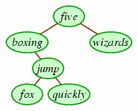
The following is an example of a binary search tree of strings using an alphabetic ordering.
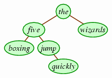
If you look at the root (the), you can see that all of the words in the left subtree precede it alphabetically, while the word in the right subtree follows it. The same holds for the other internal nodes, five and jump, and so this is a binary search tree.
The nice thing about a binary search tree is that it gives a simple technique for searching for an element — hence the name binary search tree. For example, suppose we want to determine whether the tree holds the string fox. We would start at the; since fox precedes that, we know that only the left subtree is worth searching. Then we look at the left child, five. Since fox follows five, we descend to its right child, jump. And since fox precedes jump, we know that it must be in jump's left subtree if it's in the tree at all. But it isn't, and so we have concluded that fox is not in the tree by looking at only three of the six nodes. This is a marked improvement over a linked list, where we would need to search through all of the values to see whether any of them match the query value (fox). (Saving the effort of examining just three words, as in this example, is rather underwhelming. The savings would be more dramatic if we were working with a larger tree. But using larger trees would require chopping more down to make paper for the drawings and explanations in this book. So use your imagination.)
Of course, to get a tree of some size, we want some way to add elements
into it. The simplest technique is to descend the tree just as
we search for the value to be added, and then to add the value
in place of the null reference that we reach.
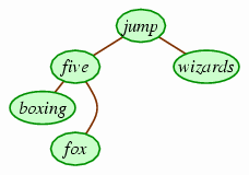
If we wanted to add fox to the above tree, for example,
we'd end up with the following.
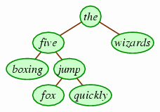
In fact, you can verify that the original tree is the result of starting from an empty tree and inserting in order the words of the sentence
(Incidentally, the sentence is a pangram,
a sentence containing all letters of the alphabet. It is four letters
shorter than the more famous pangram, the quick brown fox jumps over
the lazy dog.
)
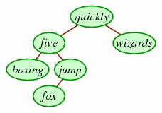
Removing a value from a binary search tree is somewhat more complicated. It's easy enough if we want to remove the value at a leaf, but how to remove an internal node is less obvious. Suppose, for example, that we want to remove the from our current binary search tree. We can't just delete the node; we would then have two trees, not one. What, then, can we do?
You may be tempted to suggest that we should simply inch up one of the children, and then inch up one of its children into that spot, and so on. If we happen to choose to raise the left child, we would end up with the following.
This is not a valid binary search tree: The left subtree of five includes some words that follow it alphabetically (jump, for instance). Of course, we could choose to raise the right child instead, and that would work on this particular tree, but it's not difficult to come up with other examples where it wouldn't.
The easiest approach is to replace the removed value with the largest value in that node's left subtree. (The smallest value in the right subtree works also.) If we did this here, we would determine that quickly is the largest value in the's left subtree, and so we would delete that leaf and place it at top.
This works well as long as the removed node in the subtree is a leaf. It may not always be a leaf, though. For example, if we remove quickly now, the largest value in the left subtree is jump, which is not a leaf. However, it conveniently has only one child, so we can instead simply connect the node that was referring to the jump node to jump's child instead.
Of course, you might suppose that we were lucky there: What if the largest node has two children? But in fact, this will never be: The largest value in any subtree of a binary search tree will always be the rightmost node. This makes it easy to find: Start at the subtree's root and proceed right until there is no right child. Of course, once we get there, it won't have a right child, although it may have a left child.
5.2.2. The TreeSet class
Given that a binary search tree is well-adapted for querying whether a particular value is contained within it, you might infer that it is a good candidate for implementing the Set ADT that we saw in Section 1.1.1. And you'd be right: In fact, the java.util package includes just such an implementation, called TreeSet.
Before we see how this can be implemented, we first need to
confront the requirement for a binary search tree that the
elements must be ordered. Though we know we can use comparison
operators (such as `<') with ints and
doubles, using them on objects is disallowed (as is
using all operators except == and !=).
To address this, Java includes the Comparable interface defining
a compareTo method.
public interface Comparable<E> {

    public int compareTo(E other);

}
The compareTo method will be called on
some object of a class implementing Comparable,
and the method will take some other object for the parameter.
Suppose we call the receiving object receiver and the
argument object argument.
receiver.compareTo(argument)
The receiver and argument will relate according to the ordering in one of three possible ways; each dictates a different return value.
receiver precedes argument |
Return some negative integer (any negative number). |
|---|---|
receiver follows argument |
Return some positive integer (any positive number). |
receiver equals argument |
Return 0. |
A few of Java's built-in classes, including String and wrapper classes like Integer, implement the Comparable interface. Of course, if you want a TreeSet of some objects of a class that you create, then your class will need to implement Comparable according to the above specification to define such an ordering. We'll see an example of this soon.
For now, though, let's look at the partial implementation of TreeSet in Figure 5.3.
Figure 5.3: A partial implementation of java.util's TreeSet class.
  1  public class TreeSet<E extends Comparable<E>> implements Set<E> {

  2      private TreeNode<E> root;

  3      private int curSize;

  4

  5      public TreeSet() { root = null; curSize = 0; }

  6

  7      public int size() { return curSize; }

  8

  9      public boolean contains(E value) {

 10          TreeNode<E> n = root;

 11          while(n != null) {

 12              int c = value.compareTo(n.getValue());

 13              if(c < 0)      n = n.getLeft();

 14              else if(c > 0) n = n.getRight();

 15              else           return true;

 16          }

 17          return false;

 18      }

 19

 20      public boolean add(E value) {

 21          if(root == null) {

 22              root = new TreeNode<E>(value, null, null);

 23              curSize++;

 24              return true;

 25          } else {

 26              TreeNode<E> n = root;

 27              while(true) {

 28                  int c = value.compareTo(n.getValue());

 29                  if(c < 0) {          // value should be in left subtree

 30                      if(n.getLeft() == null) {

 31                          n.setLeft(new TreeNode<E>(value, null, null));

 32                          curSize++;

 33                          return true;

 34                      } else {

 35                          n = n.getLeft();

 36                      }

 37                  } else if(c > 0) {   // value should be in right subtree

 38                      if(n.getRight() == null) {

 39                          n.setRight(new TreeNode<E>(value, null, null));

 40                          curSize++;

 41                          return true;

 42                      } else {

 43                          n = n.getRight();

 44                      }

 45                  } else {

 46                      return false;

 47                  }

 48              }

 49          }

 50      }

 51

 52      // `remove' and `iterator' methods omitted

109  }
The contains method, in
particular, is worth looking at. Given value for which
to search, contains uses a variable n, and each
time through the loop of line 11,
the method goes either left or right
based on whether value's compareTo says
that n's value is less than or more than
value.
The add method is a bit more complicated, but not much
more. Notice that add returns true
only if the object was actually added; since the Set
implementation is to imitate a mathematical set, the
method shouldn't add an element that is already present
(line 46).
There are two Set methods missing from Figure 5.3.
The remove method is much more complex than
add. If you're
curious, you can find an implementation of remove in
Figure 5.4, but it's pretty difficult to
untwist. The other method is the iterator method, which
we'll address in Section 7.1.4 to illustrate
a concept that will be useful in implementing it.
Figure 5.4: A
removemethod for TreeSet.public E remove(E value) {
if(root == null) return null; // no match in empty tree
E old;
int c = value.compareTo(root.getValue());
if(c == 0) { // removing root
old = root.getValue();
root = removeRootValue(root);
} else { // removing some other node
TreeNode<E> n; // will be node holding value
TreeNode<E> p = root; // always n's parent
boolean nleft = c < 0; // true when n is p's left child
if(nleft) n = p.getLeft();
else n = p.getRight();
// descend down to where n is matching node
while(true) {
if(n == null) return null; // no match found
c = value.compareTo(n.getValue());
if(c < 0) { p = n; nleft = true; n = p.getLeft(); }
else if(c > 0) { p = n; nleft = false; n = p.getRight(); }
else break;
}
old = n.getValue();
if(nleft) p.setLeft(removeRootValue(n));
else p.setRight(removeRootValue(n));
}
curSize--;
return old;
}
// takes out value at root, returning the tree following the removal.
private TreeNode<E> removeRootValue(TreeNode<E> root) {
if(root.getLeft() == null) { // if either child is missing,
return root.getRight(); // just return the other child.
} else if(root.getRight() == null) {
return root.getLeft();
} else { // root has both children, so replace
// root value with left subtree's maximum
TreeNode<E> n = root.getLeft(); // n will be left's maximum
if(n.getRight() == null) { // extract root's left child
root.setLeft(n.getLeft());
} else { // extract largest in left subtree
TreeNode<E> p = n; // always n's parent
n = n.getRight();
while(n.getRight() != null) { p = n; n = n.getRight(); }
p.setRight(n.getLeft());
}
root.setValue(n.getValue());
return root;
}
}
5.2.3. Using TreeSet
Using TreeSet with classes already defined as implementing Comparable is easy. We'll look at the case that isn't easy: Suppose we want to store objects of a custom-written class. In particular, suppose that we have a set of cities with populations, represented by a City class.
public class City {

    private String name;

    private int population;


    public City(String n, int p) {

        name = n; population = p;

    }


    // ... other methods ...

}
To be able to place City objects into the TreeSet, we need to specify that the City class implements the Comparable interface.
public class City implements Comparable<City> {
To write the compareTo method required for a Comparable
implementation,
we'll need to decide how the cities should be ordered.
Suppose that we want the TreeSet to store them in order by name.
Then we could use the following compareTo method using
String's compareTo method to compare names.
public int compareTo(City arg) {

    return this.name.compareTo(arg.name);

}
This technique has the disadvantage that any two cities with the name would be regarded as equal. We'd have to consign the Portlands (in Maine and Oregon) to a battle over who gets to keep the name. Others, like Nashville, Arkansas (pop. 4,878), might as well surrender.
TreeSet's Iterator goes through the tree using an in-order
traversal. As a result, if cities is a TreeSet storing
City objects, then we can display their names in increasing
order with the following.
for(Iterator<City> it = cities.iterator(); it.hasNext(); ) {

    System.out.println(it.next().getName());

}
This would not technically be in alphabetic order.
Instead, String's built-in compareTo method uses
We might decide to have the cities ordered by population instead.
All we have to do is to change the compareTo method.
public int compareTo(City arg) {

    return this.population - arg.population;

}
Notice the shortcut of simply subtracting two integers to get a positive number or negative number. Of course, we can still have cities that are equal according to this ordering (i.e., which have the same populations), but any battle over who gets to maintain the population can stop after the first death. (That death, though, might put the city in competition with someplace else.) We can save most of those lives by breaking ties based on the cities' names.
(This subtraction shortcut can be incorrect, though, if it results in overflow. There is no danger of this here, because no populations will be negative. But if we had both positive and negative integers, this would be a potential bug.)
5.2.4. Random search tree height (Optional)
Because the major BST operations all take time proportional to the tree's depth, it is important that we get a good feel on the efficiency of the data structure. In Section 5.1.3, we saw that a binary tree containing n values will have a height between log2 n and n. A reasonable question to ask is: If we were to insert values into the tree in random order, what would the height be?
Our answer to this question requires some fairly intense
mathematics. While none of the mathematics is particularly deep,
the argument is fairly intricate, and the techniques employed
are enlightening. Nonetheless, it is somewhat beyond the scope
of what is normally required of students studying data
structures, so this section is labeled optional.
We'd like to figure out the expected height of a randomly generated binary search tree. But determining the height of a random tree is rather difficult, for it involves determining which of the random nodes is at the maximum depth: It turns out to be more convenient to find the total depth of all the nodes in the tree. Having the total, it will be easy to find the average depth — and in fact, since trees always have more nodes toward their bottom than toward the top, the average depth is very close to the maximum depth in a typical tree.
So: Let us define Dn to be the expected total depth of a random binary search tree with n nodes. Of course, we know that D0 is 0 and D1 is 1. That is easy. But defining Dn for larger n is somewhat more difficult. Here's the expression:
What's going on here is that in a random binary search tree with n elements, each element is equally likely to be the root — with a probability 1/n. So we're summing over each possible root element i of 1/n times the expected total depth of the tree with i at the root. To get the expected total depth of the tree, we divide our computation into three parts:
There are i − 1 nodes that will be in the subtree to the left of i, in a random order. The value of Di − 1 represents the total depth of the subtree rooted at the left child of i, and in the overall tree each of these nodes is one deeper than they are in the left subtree alone, since the path to each also goes through i. Thus, the total depth of all nodes in the left subtree is (i − 1) + Di − 1.
The depth of node i is simply 1.
There are n − i nodes that will be in the subtree to the right of i. By the same argument that we had for the left subtree, the total depth is (n − i) + Dn − i.
Let us simplify Dn.
| Dn | = | ∑i = 1n (1/n) (((i − 1) + Di − 1) + 1 + ((n − i) + Dn − i)) |
| = | ∑i = 1n (1/n) (((i − 1) + 1 + (n − i)) + Di − 1 + Dn − i) | |
| = | ∑i = 1n (1/n) (n + Di − 1 + Dn − i) |
Incidentally, you can notice that this expression is roughly the same as the expression for the expected amount of time for Quicksort: After picking i as the pivot, we would take O(n) time to partition the elements, and then we would recurse on the i − 1 elements less than i and on the n − i elements more than i. Thus, our proof for the total depth of a random tree will work exactly the same as a proof for the expected time for Quicksort.
We'll prove, in fact, that Dn < 2 n Hn, where Hn is defined as the nth harmonic number:
Note that we are proving an upper bound on Dn — that Dn is less than something. In fact, it is possible to prove Dn is precisely 2 n Hn − 3 n + 2 Hn, but proving this is much more tedious, and all we really care about is an upper bound on the total depth.
Our proof that Dn < 2 n Hn proceeds by induction. First, the base case: We have already noted that D1 = 1, which is indeed less than 2 ⋅ 1 ⋅ H1 = 2 ⋅ 1 ⋅ 1 = 2. The bulk of the argument lies in the induction step. Suppose that we know for all k between 1 and n − 1 that Dk < 2 k Hk. We'll now begin in trying to prove that this implies Dn < 2 n Hn.
| Dn = ∑i = 1n (1/n) (n + Di − 1 + Dn − i) | = | (1/n) ∑i = 1n (n + Di − 1 + Dn − i) |
| = | (1/n) (∑i = 1n n + ∑i = 1n Di − 1 + ∑i = 1n Dn − i) | |
| = | (1/n) (n² + ∑i = 1n Di − 1 + ∑i = 1n Dn − i) |
Now we know that D0 is 0, so we'll knock out those items from the summation; and then we'll shift the indices on the first summation down one and reverse the second summation without changing their values.
| Dn = (1/n) (n² + ∑i = 1n Di − 1 + ∑i = 1n Dn − i) | = | (1/n) (n² + ∑i = 2n Di − 1 + ∑i = 1n − 1 Dn − i) |
| = | (1/n) (n² + ∑i = 1n − 1 Di + ∑i = 1n − 1 Di) |
Now the two summations are identical, so we can combine them. From here we can simplify and then apply our assumption for the induction step that Dk < 2 k Hk for k between 1 and n − 1.
| Dn = (1/n) (n² + ∑i = 1n − 1 Di + ∑i = 1n − 1 Di) | = | (1/n) (n² + 2 ∑i = 1n − 1 Di) |
| = | n + (2/n) ∑i = 1n − 1 Di | |
| < | n + (2/n) ∑i = 1n − 1 2 i Hi | |
| = | n + (4/n) ∑i = 1n − 1 i ∑j = 1i (1/j) | |
| = | n + (4/n) ∑i = 1n − 1 ∑j = 1i (i/j) |
Now for the trickiest step: Note that the double-summation looks like the following:
| i = 1: | 1/1 | ||||||||
| i = 2: | 2/1 | + | 2/2 | ||||||
| i = 3: | 3/1 | + | 3/2 | + | 3/3 | ||||
| i = 4: | 4/1 | + | 4/2 | + | 4/3 | + | 4/4 | ||
| : | : | : | : | : | : | ||||
| i = n − 1: | (n − 1)/1 | + | (n − 1)/2 | + | (n − 1)/3 | + | (n − 1)/4 | + … + | (n − 1)/(n − 1) |
Essentially, our double-summation is adding up all the entries in this matrix by row — but to continue our proof we'll rearrange our summation to add up the same entries by column. Note that the jth column has j in all the denominators, and the numerators range over all the i between j and n − 1.
| Dn < n + (4/n) ∑i = 1n − 1 ∑j = 1i (i/j) | = | n + (4/n) ∑j = 1n − 1 ∑i = jn − 1 (i/j) |
| = | n + (2/n) ∑j = 1n − 1 (2/j) ∑i = jn − 1 i |
Using the popular identity ∑i = 1k − 1 i = (k − 1) k / 2, we can continue.
| Dn < n + (2/n) ∑j = 1n − 1 (2/j) ∑i = jn − 1 i | = | n + (2/n) ∑j = 1n − 1 (2/j) (∑i = 1n − 1 i − ∑i = 1j − 1 i) |
| = | n + (2/n) ∑j = 1n − 1 (2/j) (((n − 1) n)/2 − ((j − 1) j)/2) | |
| = | n + (2/n) ∑j = 1n − 1 ((n − 1) n ⋅ (1/j) − (j − 1)) | |
| = | n + (2/n) ((n − 1) n (∑j = 1n − 1 (1/j)) − (∑j = 1n − 1 j) + (∑j = 1n − 1 1)) | |
| = | n + (2/n) ((n − 1) n Hn − 1 − ((n − 1) n)/2 + (n − 1)) | |
| = | n + 2 (n − 1) Hn − 1 − (n − 1) + 2 (n − 1) / n |
At this point we'll factor out 2 (n − 1) from the second and last terms. Note that Hn = Hn − 1 + 1/n.
| Dn < n + 2 (n − 1) Hn − 1 − (n − 1) + 2 (n − 1) ⋅ (1/n) | = | 2 (n − 1) (Hn − 1 + 1/n) + n − (n − 1) |
| = | 2 (n − 1) Hn + n − (n − 1) | |
| = | 2 n Hn − 2 Hn + 1 |
Now since n ≥ 1, 2 Hn will be at least 2. We use this as we continue.
| Dn < 2 n Hn − 2 Hn + 1 | ≤ | 2 n Hn − 2 + 1 |
| < | 2 n Hn |
Thus, we have the inductive step: If Dk < 2 k Hk for 1 ≤ k < n, then this implies that Dn < 2 n Hn. Dn < 2 n Hn By induction, then, we have Dn < 2 n Hn for all n.
The total depth of all nodes is 2 n Hn for a randomly created n-node binary search tree. This means that the average depth of each node is 2 Hn. We saw in an earlier footnote that Hn is at most 1 + ln n. Thus, the average depth of a node in a random binary search tree is less than 2 (1 + ln n).
5.3. Red-black trees
Though a random
binary search tree would have O(log n)
height, in practice binary search trees are not random. In fact,
people quite often enter data in increasing order, and
adding them into a TreeSet as implemented earlier would result in a
tree whose height is n.
Consequently, all the major methods (contains,
add, remove) would end up taking O(n) time.
This is quite a blow when we are hoping for O(log n) running
time.
Fortunately, there is a way to guarantee that the binary search tree's height (and hence the running time of the major operations) is O(log n). In fact, java.util's TreeSet class as it is actually implemented uses just such a technique, called red-black trees.
Implementing red-black trees is rather tricky; we won't look at the Java code implementing it. But the basic concept underlying it is relatively simple to understand.
5.3.1. The red-black invariant
We'll think of every node of the tree as being colored
either red
or black; additionally, we'll consider all the null references
in a tree to be black. Tracking nodes' colors is relatively simple:
We can just add an additional boolean instance variable to
the TreeNode class for indicating whether a node is black or not.
As we manipulate the tree, our invariant will be that we maintain the following two constraints concerning the node colors:
- The red constraint: Red nodes' children must be black.
- The black constraint: Every path from the root to a
nullreference must contain the same number of black nodes.
Consider the three example colorings below; the red nodes are
drawn in pink. The null
references appear as tiny black dots.
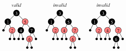
The first tree is a red-black tree: You can verify that each of
the three red nodes has only black children, and that the path
from the root to any of the null references contains
three black nodes (counting the null reference as a
black node). The second tree satisfies the black constraint
but fails the red constraint: One of the red nodes (7) has a red child (6).
The third tree illustrates an attempt to fix this by coloring
the 6 node black; this succeeds in passing the red constraint,
but now it fails the black constraint: A path from the root
to either of 6's null references contains four black
nodes, but a path from the root to any of the other null
references (such as 7's right child) contains only three.
Given a tree, determining a legal red-black coloring can be
relatively tricky. Sometimes, in fact, it is impossible:
Consider a tree where one null reference's
depth is d and another null reference's depth is more
than 2 d.
According to the red constraint, each red node down the path
to the second null must be followed by a black child; thus,
at least half of the more than 2 d nodes — that is, more than
d of them — must be black.
But according to the black constraint,
the number of black nodes on each path must be at most d,
because there are only d nodes on the
path to the first null reference.
Thus, the two constraints cannot both be satisfied
simultaneously for such a tree.
To summarize: The depth of any null reference in a red-black
tree cannot exceed twice the depth of the shallowest null
reference.
The depth of the deepest null reference is the height
of the tree, which corresponds to the total amount of time for
the major operations.
We claim that this height must be at most
2 log2 n for a
red-black tree of n nodes.
Suppose this were not the case — that is, the depth of some
null reference is more than
2 log2 n.
According to the previous paragraph, this would mean
that the shallowest null reference has a depth of more
than log2 n; all the levels at depths smaller than this (that is,
depths less than or equal to log2 n) would have to be
complete. We've already seen that when a complete level at depth
d has 2d nodes. As a result,
the number of nodes at depths less than or equal to log2 n would
be
1 + 2 + … + 2log2 n = 1 + 2 + … + n, which exceeds the n
nodes that our tree has.
This contradiction means that the deepest null
reference — and the height of the tree — must be at most
2 log2 n.
5.3.2. Maintaining the invariant
While we understand what a red-black tree is, and why it must have a height of O(log n), this is not enough to establish that the data structure is truly viable: We also need to know that it is indeed possible to maintain the invariant as we add and remove values in the tree. Preferably, we would also like a technique for maintaining the invariant efficiently — that is, taking O(log n) time.
We'll see how this can be done with inserting values through an example of starting with an empty tree and successively adding the numbers 1 through 6; as we go through the example, we'll see that the technique developed can be used for inserting values into any red-black tree.
Each time we insert a value, we'll insert it as a new node in
place of an existing null reference, just as with
inserting into a simple binary search tree. The new node created
will be a red node.
Adding the first node presents no problems: We end up with a red
node with two black null references, consistent with
both constraints.
When we add 2 in its proper place within the binary search tree, we arrive at a problem that we'll confront repeatedly: Although adding a new red node will never introduce problems with the black constraint, it can cause problems with the red constraint. In particular, the new node's parent may also be red; if this is the case, then we need to find a way to manipulate the tree to repair it so that it still satisfies the binary search tree and red-black tree invariants. Our solution will sometimes involve performing a sequence of several manipulations; we will, however, maintain the following invariant.
Red-black insertion invariant: The tree fully meets the binary search tree invariant and the black constraint. The red constraint is satisfied everywhere except possibly for one red node — which we'll call the offender — which has one red child.
In the following diagrams, we'll use an arrow to point to the offender.
Continuing, then, with inserting 2, we would initially not meet the red constraint, as indicated at left below. The diagrams will include a small arrow pointing to the offender (node 1 in the tree at left).
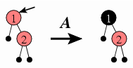
For each such situation, we need to identify a way of repairing the offender to satisfy the red constraint. In this case, the fix is simple: We can just color the offender black. We'll call this Case A, which is denoted in the diagram above with an A above the transformation arrow.
Case A: If the offender is the tree's root, then we color it black and end the insertion process.
Although coloring the offender black will always remove all problems with the red constraint, it can introduce problems with the black constraint because this will change the number of black nodes along paths to leaves. When the offender is the root, though, coloring it black is OK: All paths had an equal number of black nodes before the recoloring, and coloring the root black will add one black node to all of these paths — but they will still all have an equal number of black nodes.
Adding 3 will introduce a new problem: Now the offender isn't the root, so Case A doesn't apply. We need a new way of addressing this.
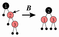
This inspires Case B.
Case B: If the offender's sibling is black, then the tree rooted at the offender's parent will match one of the four trees on the left side of the below diagram. We will rearrange the nodes to match the right side, and we end the insertion process.
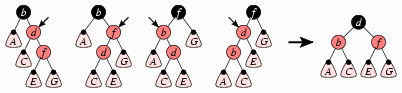
The four trees at left represent the four possible arrangements of the offender with respect to its parent and its right child; the offender is always pointed to by a small arrow. The rounded triangles represent subtrees, and the small black circle at the top of each subtree indicates that it has a black root. Just after inserting 3 above, the first tree is the matching tree, and each subtree in the diagram is just a simple
nullreference.We need to satisfy ourselves that the four trees represent all the possible trees that we might have whenever our tree satisfies the insertion invariant and the offender's sibling is black (as Case B requires). You can see that the four cases correspond to the different possible arrangements of the offender's parent, the offender, and the offender's red child; but implicit in the diagrams is an assumption that the offender's parent and the root of each subtree must be black. We know that the offender's parent must be black because if it were red, it would violate the red constraint, and our invariant only allows the offender to have a red child; the topmost subtree must have a black root because the offender's sibling must be black for Case B to apply; the root of the offender's other subtree must be black, because the insertion invariant requires that the offender have only one red child; and the red child must have black children because it does not violate the red constraint.
In this case, the tree matches the first of the four subtrees at
left, and the subtrees are all simply null references;
we manipulate it to match the tree at right.
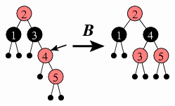
Adding 4 introduces the last case that we need to address: Here, the offender isn't the root, and its sibling is red.
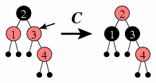
For this, we need Case C.
Case C: If the offender's sibling is red, then we color both the offender and its sibling black instead, and we color the offender's parent red. If the offender has a grandparent, then coloring the offender's parent red may violate the red constraint for the grandparent; if so, we repeat the repairing process with the offender now being the grandparent.
This is the only case that may require continuing the insertion process. In the case of adding 4, however, this is not an issue, since the offender 3 does not have a grandparent.
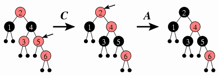
Observe that these three cases cover all the possibilities: Either the offender is the tree's root (Case A) or it has a sibling, which will be either black (Case B) or red (Case C). Thus, we won't need to introduce any new cases as we continue with inserting numbers. We see another application of Case B when we insert 5.
And in inserting 6, we see a case where we apply Case C once and then Case A.
This, then, is the insertion algorithm: We insert the new value
in a newly created red node at the tree's bottom, and then we
manipulate the tree if necessary so that it fulfills the red
constraint. You should see that this takes O(log n) time:
The first insertion step will take O(log n) time to descend
to the appropriate location at the tree's bottom. Determining
whether we need to perform a manipulation and then performing it
takes O(1) time; this will require a parent instance
variable for each TreeNode so that we can quickly determine a
node's parent, but maintaining the parent references'
consistency won't present any problems.
We may need to perform multiple manipulations (in particular,
when we perform Case C); but in each case, the next
offender is the previous offender's grandparent.
Because we are moving up the tree each time, we won't
have to perform more than O(log n) of these manipulations,
each of which takes O(1) time.
Thus, the repairing process take O(log n) time,
and so the overall insertion process takes O(log n) time.
Deleting a value from a red-black tree is even more complex than inserting a value. We won't examine it; suffice it to say that it, too, takes O(log n) time.

Data & Procedure is licensed under a Creative Commons Attribution-Share Alike 3.0 License.
Based on a work at http://www.cburch.com/books/data/.