While the technique as stated here is
theoretically correct, this implementation has a major bug.
Suppose we want to find the
square root of 100,000, for example. This code will start by squaring
half of that (50,000), and the result will be overflow
— a number larger than an int can handle.
This implementation is correct only for integers up to 92,680.
By contrast, isqrtIncrement is correct for integers up to
2,147,395,599. For this chapter,
however, we'll ignore such issues.
Chapter 4. Reasoning about efficiency
When we face a computational problem, of course we first want to find a correct algorithm for solving it. But given a choice between several correct algorithms, we would also like to be able to choose the fastest among them. Analyzing algorithms' performance is the subject of this chapter. After seeing the basic technique for theoretical analysis, called big-O notation, we'll look at its application to analyzing algorithms' speed for two significant problems: sorting arrays and counting primes. We'll conclude by looking at how the same concept can be applied to analyzing algorithms' memory usage.
4.1. Analyzing efficiency
Suppose, for example, that we want to write a program to determine integer square roots, which we'll define as the largest integer whose square does not exceed the query integer (in mathematical notation, ⌊sqrt(n)⌋). For example, the integer square root for 30 is 5, since 5² ≤ 30 but 6² > 30; for 80, it is 8; and for 100, it is 10.
The first technique one might imagine is this: We'll square consecutive numbers until we pass the query integer. Then we'll return one less than that.
public static int isqrtIncrement(int query) {

    int cur = 0;

    while(cur * cur <= query) cur++;

    return cur - 1;

}
Another technique is based on binary search: We'll maintain a range where we think the integer square root might be; and each iteration, we'll halve the range so that it still spans the integer square root, but one end of the new range is at the old range's midpoint.
public static int isqrtHalve(int query) {

    int low = 0;          // invariant: low * low <= query

    int high = query + 1; // and high * high > query

    while(high - low > 1) { // while range has >1 number

        int mid = (low + high) / 2;

        if(mid * mid <= query) low = mid;

        else                   high = mid;

    }

    return low;

}

Which approach is faster? The answer may not be obvious looking at the code alone.
One way to determine this is to implement both algorithms and test. To do this, I wrote both and used them to find the sum of the integer square roots of the integers up to 90,000.
isqrtIncrement326 ms isqrtHalve43 ms
While this answers the question at hand, the answer is not
entirely satisfying: Other than that
isqrtHalve is faster than than isqrtIncrement,
what have we learned? All we have is a single result, without
much feeling for why one is faster than the other.
We would like a handle on the reason for the difference for
several reasons:
We'd like to be confident that the results obtained aren't peculiar to the particular computer on which we happened to run the tests.
We'd like to be confident that the results aren't peculiar to the specific tests that we ran. Here, we should be pretty confident: The algorithms are both pretty simple, so we don't expect them to behave peculiarly in some cases. Moreover, the input is simple enough that we can test a very wide range of possible inputs.
By contrast, if we wanted to analyze a program to sort an array, we'd need to try all different ways to arrange each array, on the off-chance that one of those ways happens to be a very bad case for the program. Testing such a program on such a large number of possible inputs would be prohibitive.
We'd like to have a feel for the algorithms' weaknesses. If we can identify a bottleneck, then that gives us some insight where we should work hardest to improve performance — in effect,
widening
the bottleneck. The resulting algorithm may be faster than anything we thought of previously.
For all these reasons, we'd like a different way to think about the efficiency of a program.
4.1.1. Big-O notation
What we'll do is to imagine a graph of how the algorithm works relative to how big the input is. Actually, for just this example, we won't just imagine it: I'll draw it for you. You can see it in Figure 4.1. (Actually, this graph is not the true graph. The original graph based on the actual data was quite bumpy, and I smoothed it out to convey the methods' essential behavior. The bumps, as you see, did not entirely disappear.) I want you to appreciate all the time I've saved you: Measuring all those times to get that graph is quite a pain. Luckily, we won't have to do this manually again.
Figure 4.1: Comparing two square root algorithms experimentally.
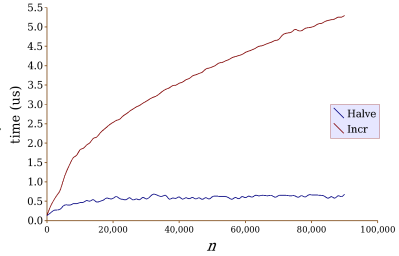
When you look at the graph, you see something quite noticeable.
Not only is isqrtIncrement much slower than
isqrtHalve for large n, but the difference increases
dramatically as n increases. In fact, the isqrtHalve curve looks almost flat
at its large end, while isqrtIncrement's curve
continues to increase, though the rate of increase is slowly
slowing as n grows.
In fact, what we're looking at here is the difference between an
inverse parabola (i.e.,
f(n) = a sqrt(n) + b)
and a logarithmic
curve (i.e.,
f(n) = a (log n) + b).
With an inverse
parabola, quadrupling n doubles the value
(a sqrt(4 n) = 2 a sqrt(n)),
neglecting the y-intercept
(b). You can see that isqrtIncrement follows this
behavior: At n = 20,000, the time is
2.5 μs, whereas with n = 80,000, the time
is double that, 5 μs.
However, quadrupling n with isqrtHalve has hardly
any effect at all on the time: At n = 20,000,
the time is
0.58 μs, whereas at n = 80,000,
the time is 0.66 μs.
The curve for isqrtHalve starts out growing, but it
quickly becomes very close to flat; this is characteristic
of a logarithmic curve, which this happens to be (though with
some noise added).
Any algorithm whose behavior is characterized by an inverse parabola will eventually be much slower than an algorithm characterized by a logarithmic curve. It doesn't matter what the coefficient a and the y-intercept b are for the two curves: These values affect the exact crossover point, but no matter what, the inverse parabola will eventually surpass the logarithmic curve. (Well, it matters that a is positive. But it will be positive, since algorithms will be slower as n increases.)
We can actually visualize a whole hierarchy of different curves. For example, if we have another algorithm whose graph is linear, it will eventually raise above one characterized by an inverse parabola. (The inverse parabola, after all, slowly decelerates, whereas a line always grows at the same rate.) And a parabola, which is continually accelerating, would eventually go above a line.
We can tabulate this hierarchy.
slowest parabola f(n) = a n² + b line f(n) = a n + b inverse parabola f(n) = a sqrt(n) + b logarithmic curve f(n) = a (log n) + b
Computer scientists have a way of talking about these — and
other — curves called hiding
any constant multipliers, as well as any
lower-order terms.
Note that this means that not only is
a n² + b
classified as O(n²): So is
a n² + b n + c
and
a n² + b sqrt(n) + c.
(You may be wondering how to pronounce this.
Some people read O(log n) as
big-O of log n;
others say,
order log n.
Both are correct.)
This terminology generalizes to other functions, too. While we don't have an English term for a O(n1.5) curve, big-O notation gives us a way to talk about that function anyway. By the way, it ranks somewhere between O(n) and O(n²).
In fact, the big-O bound is technically an upper bound. Thus, we can legally say that a line (which is O(n)) is O(n²) — or even that it is O(nn). This fact is important, because sometimes the nature of a curve is difficult to determine exactly, and so to get a result we may end up needing to cut some corners in our analysis by overestimating a bit. We'll see some examples of this later in this chapter, particularly in Section 4.3.
In talking about algorithms, we use this phrasing:
With the ranking of
different functions internalized, we understand this
as a fancy way of saying that isqrtHalve takes O(log n) time, while
isqrtIncrement takes O(sqrt(n)) time.isqrtHalve is much better
than isqrtIncrement — at least for large
n. (We're not so worried about small n here,
because both algorithms are quite fast for small n anyway. It
may be that
isqrtIncrement is faster there, but since we're talking
about fractions of a microsecond for small n in any case,
distinguishing which is faster there isn't important.)
You might be wondering: What if we have two O(sqrt(n)) algorithms? Big-O analysis won't indicate which is faster, since big-O notation hides those constant coefficients. Unfortunately, there's no clean way around this: Those constant coefficients will depend on the particular computer for which we implement the algorithms, and they'll be very different for another computer. In fact, one of the O(sqrt(n)) algorithms may be faster on some computers, while the other is faster on other computers. But if we have a O(sqrt(n)) algorithm and a O(log n) algorithm, we know that regardless of the computer we choose, the O(log n) algorithm will be faster for large n.
Now, here's the important part: With just a bit of practice, we can look at an algorithm and quickly tell what its big-O bound is. We don't need to go through all the bother of programming it up, taking lots of measurements, drawing a graph, and then simply guessing what the curve looks like.
Let's take the isqrtIncrement method as a simple
example.
public static int isqrtIncrement(int query) {

    int cur = 0;

    while(cur * cur <= query) cur++;

    return cur - 1;

}
You can look at this and immediately see that we'll go through the
loop for at most sqrt(n) + 1 iterations.
Each iteration takes some constant a amount of time — some
amount of time to test whether cur * cur <= query, and
some other amount of time to increment cur.
Thus, the loop will take
a (sqrt(n) + 1)
time. In addition to this, there will be another constant b
amount of time incurred once only: This will be the time to create the
cur variable initialized to 0, to make the final test
cur * cur <= query after the final iteration, and to
subtract 1 from cur at the end.
Thus, isqrtIncrement takes at most
a (sqrt(n) + 1) + b
= a sqrt(n) + (a + b)
= O(sqrt(n))
time for some constants a and b
whose values depend on the particular compiler and computer
used.
We can apply similar reasoning to isqrtHalve.
public static int isqrtHalve(int query) {

    int low = 0;          // invariant: low * low <= query

    int high = query + 1; // and high * high > query

    while(high - low > 1) { // while range has >1 number

        int mid = (low + high) / 2;

        if(mid * mid <= query) low = mid;

        else                   high = mid;

    }

    return low;

}
The biggest difficulty here is determining the number of
iterations for the loop. To get a handle on this, notice that
the quantity high - low, which starts at
query + 1, will halve each time.
It doesn't quite halve: If high - low is odd, then
the midpoint will
be closer to low than to high, and if it
happens to be low that is changed to mid, then
the quantity high - low becomes ½ more than half what
it was. (Of course, it would be ½ less than half if
high is the variable changed to mid.)
If we were going to be completely rigorous, we might
argue that the quantity high - low goes down by at least
one third with each iteration. But we won't let such nitpicking
muddy our argument here.
We can tabulate, then, where high - low will be after
each of the first few iterations.
iterations high - low0 query+ 11 ( query+ 1) / 22 ( query+ 1) / 43 ( query+ 1) / 84 ( query+ 1) / 16
In general, after k iterations, high - low will be at
(query + 1) / 2k.
The method stops once this quantity reaches 1, which leads to the below
equation; we have only to solve that equation for k to arrive at the
number of iterations.
(query+ 1) / 2k = 1
query+ 1 = 2k
log2 (query+ 1) = k
Thus, the loop will stop after
log2 (query + 1) iterations.
In general, whenever we have a loop that stops once a quantity
reaches a constant, and that quantity starts at x and
decreases by a constant
percentage with each iteration, the loop will stop after
O(log x) iterations.
By the way, you might have noticed that the logarithm's base disappeared. We write O(log n) rather than O(log2 n). This is because the logarithm's base, when it is constant, is unimportant: The well-known logarithmic identity loga x = (logb x) / (logb a) says that changing the logarithm's base from one constant a to another constant b simply changes the coefficient by 1 / logb a. Since big-O notation hides constant coefficients anyway, the base is irrelevant, and we might as well omit it.
Big-O analysis allows us to approximate and compare algorithms' performance without actually implementing them. While it only provides the roughest estimate of running time, that estimate works out well when we are concerned with performance for very large inputs.
4.1.2. Multiple loops
To become more familiar with using big-O notation, we need to examine more examples. The examples above were fairly simple, involving only a single loop. Often, however, algorithms involve multiple loops. Consider the following example intended to test whether all of the integers in an array are unique.
public static boolean areAllUnique(int[] a) {

    for(int i = 0; i < a.length; i++) {

        for(int j = i + 1; j < a.length; j++) {

            if(a[i] == a[j]) return false;

        }

    }

    return true;

}
For each integer in this array, this method looks at all the
integers following that one (note that j starts at
i + 1) to see if any match it. If the inner loop finds
a match, then it can return false; but if there are none
found, then the outer loop continues to the next integer.
Note that in this example, the input is an array, not a number. When we want to analyze the speed of operations on an array, it is typically expressed in terms of the array's length. We'll use n to refer to the length.
One way to analyze the speed of methods using multiple loops is
to start at the innermost level and move outwards.
In this case, we can determine that the loop over j
involves at most n iterations for each i,
where n is the array's
length, and each iteration of that loops takes O(1) time.
(Often, the number of iterations is much less than n,
but remember that we are willing to overestimate with big-O
notation. In this case, as it happens, the average number of
iterations is n / 2, and the constant multiplier
½ won't
show up in the big-O bound anyway.)
Thus, the inner loop (over j) takes a total of O(n)
time it is executed. Executing this loop constitutes the whole
of each iteration of the outer loop (over i), which
involves at most n iterations. Thus, the outer loop will take
at most
n ⋅ O(n) = O(n²) time. The final return
statement will take an additional O(1) time, so the total
time taken is
O(n²) + O(1) = O(n²).
Multiple loops don't always mean that we multiply the number of iterations per loop, though. Consider the following simple method which finds the average of an array and then replaces each number that exceeds the average with the average instead.
public static void cutLargeNumbers(int[] a) {

    int total = 0;

    for(int i = 0; i < a.length; i++) total += a[i];

    int average = total / a.length;

    for(int j = 0; j < a.length; j++) {

        if(a[j] > average) a[j] = average;

    }

}
In this case, the loops are not nested, so the amount of time is the time for the first loop, followed by the time for the second loop. Here, the first loop will take O(n) time (since each of the n iterations takes O(1) time), and the second loop will take O(n) time (since each of the iterations also takes O(1) time). The pieces in between each take O(1) time, so the total is O(1 + n + 1 + n) = O(n).
This type of analysis restricts itself to two questions: What is the maximum amount of time that each iteration of the loop can take? And what is the maximum number of iterations for the loop? With these two values, then we can multiply them together to get the total time for the loop. If we have one loop nested within another, then this leads to multiplication of the numbers of iterations; and if one loop is entirely after another, this leads to addition of their running times.
This technique is sound, but sometimes it ends up overcounting, particularly if the maximum time per iteration is much more than the average time per iteration.
Consider, for example, the problem of computing the number of lattice points within a circle — that is, the number of points whose coordinates are both integers. A circle of radius 5, for example, contains 69 lattice points, as drawn below.

We will count the lattice points by first determining the number within the upper quadrant, counting those on the x-axis but not on the y-axis — i.e., those in the darkened box above. We can then multiply this by 4, to take care of the other quadrants (the lightened boxes), and then we can add 1 to account for the origin. Here is the code.
// Count integer-coordinate points in radius-r circle

public static int countLatticePoints(int r) {

    int count = 0;

    int y = 0;

    for(int x = r; x > 0; x--) {

        while(x*x + y*y < r*r) y++;

        count += y;

    }

    return 4 * count + 1;

}
A simple analysis of this code is that the inner loop will always iterate at most r times before x² + y² exceeds r². Thus, the inner loop takes O(r) time. The outer loop has r iterations, giving a total of O(r²) time.
While technically correct, O(r²) is not the best possible bound for this code. In particular, since y begins at 0 at the method's beginning and never decreases, the total number of iterations of the inner loop — across all iterations of the outer loop — is r. Thus, the total amount of time spent on the inner loop during the method is O(r); and the total time spent on the outer loop, excepting the inner loop, is O(1) per iteration, over r iterations for a total of O(r). Thus, the total time for the loop is O(r).
4.2. Case study: Sorting an array
Sorting a list is one of the most fundamental problems in computer science. The basic problem is this: Suppose we have a list of numbers.
We want to reorder the list so that the numbers appear in increasing order.
Sorting is fundamental to computer science for several reasons: First, real programs often need to sort data; second, sorting techniques prove to be a foundation for many other computational problems; and finally, the problem is relatively simple to analyze, but still complex enough to have some worthwhile intricacies. Thus, it is a perfect showcase problem for study and research.
4.2.1. Simple algorithms
There are many reasonable ways to approach the problem of
sorting an array. Most of the obvious ones are also relatively
easy to analyze. Take, for example, the
Then we find the smallest element right of the first position and swap it into the second position.
Then we find the smallest element right of the second position and swap it into the third position.
We continue doing this, each time determining the proper number to place in the next position of the array, until we've completed the array.
Writing this in a program is relatively straightforward.
public static void selectionSort(int[] data) {

    for(int i = 0; i < data.length; i++) {

        int min = i;

        for(int j = i + 1; j < data.length; j++) {

            if(data[j] < data[min]) min = j;

        }

        int t = data[min];

        data[min] = data[i];

        data[i] = t;

    }

}
We use a variable i to track which position we are
currently trying to swap into. To determine where we should
swap from, we use a variable j that steps through
every index above i, and every time we find a smaller
element, we change min to refer to that element's
index. After going through the inner loop over j's,
then, min will hold the index of the smallest number
in position i or beyond. This is the position that we
swap with position i. Then we can proceed to the
next i.
In terms of running time, selection sort isn't very difficult to analyze. Each time we reach the inner loop, it takes O(n) time (at most n iterations, each taking O(1) time), and so each iteration of the outer loop takes O(n) time. There are n iterations of the outer loop, and so the total time for selection sort is O(n²).
(You might object that using n as a bound for the inner loop's iterations is crude, and that this could affect the running time. You'd be right. But, in fact, n / 2 iterations of the outer loop involve at least n / 2 iterations of the inner loop, so the total time is at least O((n / 2)²) = O(n² / 4) = O(n²). In this case, then, the crude approximation yielded the best possible result anyway.)
Segment starts with first element only. Then we grow it to the first two elements. Then the first three elements. Then the first four elements. … until the segment covers the entire array.
Each time we want to expand the segment by an element, the only thing we need to do is to insert the new element into the already sorted list — hence the name insertion sort. The insertion process involves shifting the elements of the old segment that are greater than the new element up by one position, to make room for the new element's proper position.
To implement this in a program, we need a variable to keep
track of how large the current segment is; we'll use
i for this. Each iteration, our goal is to increment
i by one, which requires us to insert element
i into the first i elements. To shift
elements upward to make room, we'll use another variable,
j, which will start at i − 1 and
move down until element j is less than element
i.
public static void insertionSort(int[] data) {

    for(int i = 1; i < data.length; i++) {

        int t = data[i];

        int j = i - 1;

        while(j >= 0 && data[j] > t) {

            data[j + 1] = data[j];

            j--;

        }

        data[j + 1] = t;

    }

}
Analysis of the speed of this algorithm proceeds similarly to
that for selection sort: The inner loop takes a total of O(n)
time (since j may have to go from
n − 2 all the way down to 0), and there will be n − 1 iterations
of the outer loop, for a total of O(n²) time.
One difference from selection sort is that insertion sort will sometimes go faster than at other times. As an extreme example, for arrays already in sorted order, there will be never be any iterations of insertion sort's inner loop, and so insertion sort will take O(n) time. This is unusual, though. For most orderings, insertion sort takes O(n²) time. Still, since there's a chance that it may go faster, programmers generally prefer insertion sort over selection sort.
4.2.2. Mergesort
The selection sort and insertion sort algorithms, along with most other intuitive techniques, take O(n²) time. It turns out, though, that a different algorithm called Mergesort does better.
The
1. We start with an array. 2. Divide the array into two halves. and
3. Recursively sort both halves. and
4. Merge the sorted halves.
Implementing Mergesort, as done in Figure 4.2,
is really not too complex. Our method will
take two indices as parameters, start and stop,
representing which segment of the array to be sorted;
this is so that the recursive calls can specify which segment to sort.
These indices represent the first index inside the segment, and the
first index after the segment.
Figure 4.2: The Mergesort algorithm.
// Sorts the segment start..(stop-1) of the array data.

public void mergeSort(int[] data, int start, int stop) {

    if(stop - start <= 1) return;         // Base case: <= 1 element

    int mid = (start + stop) / 2;         // Determine split point

    mergeSort(data, start, mid);         // Recursively sort first

    mergeSort(data, mid, stop);             //   and second half.


    int[] other = new int[stop - start]; // Merge into another array.

    int i = start; int j = mid;    // (track position in both halves)

    for(int k = 0; k < other.length; k++) {

        if(j >= stop || (i < mid && data[i] < data[j])) {

            other[k] = data[i]; // (copy element of first array over)

            i++;

        } else {

            other[k] = data[j]; // (copy element of second array over)

            j++;

        }

    }


    for(int k = 0; k < other.length; k++) {

        data[start + k] = other[k];         // Copy other array back.

    }

}
Dividing the array into two and recursively sorting both halves
is simply a matter of finding where to split the segment (index
mid) and making the recursive calls. The bulk of the
implementation is spent in the merging. Here,
we use two indices, i and j, referring to how
far we've merged elements from the two half-segments.
We copy elements from the half-segments into another array,
each time incrementing i or j, until the
other array is filled.
Finally, we copy all the elements from the merged array back
into the original.
Analyzing the speed of Mergesort involves analyzing the speed of a recursive algorithm, something we haven't seen before. For this, we'll first analyze the total amount of time neglecting the recursive calls. In the case of Mergesort, aside from the two recursive calls, the time is spent almost entirely within the merge and copy loops. If the incoming array has n elements, then the merge loop will involve n iterations, each taking O(1) time, and the subsequent copy loop will also involve n iterations, each taking O(1) time. The total is O(n + n) = O(n). This means that for some constant c, the time taken in Mergesort, aside from recursive calls, is at most c n.
Of course, we need to include the time spent in recursive calls, too. To do this, we'll draw a recursion tree, writing for each node the amount of time spent inside that node — which we've just argued is c times the length of the array to be sorted in that node. The total amount of time spent will be the total of the times inside the nodes.
Figure 4.3 diagrams the recursion tree for an array of eight elements, echoed to the right with the time spent inside each node.
Figure 4.3: Analyzing Mergesort's performance.

We want to find the sum of these times. As it happens, the easiest way to compute this sum is to compute the sum for each level of the tree (c n) and to multiply this by the number of levels (4 in this case, but for general n it is 1 + log2 n). Thus, the total amount of time for Mergesort is at most c n (1 + log2 n) = O(n log n).
A O(n log n) bound on speed is much better than a O(n²) bound, because the value of log n will be quite small even for very large n. If n is a million (106), for example, log2 n will be roughly 20. Thus, n log n would be roughly 20 billion (2 × 10⁷), while n² would be a trillion (1012) — far, far more. Mergesort happens to be slower than insertion sort or selection sort for small arrays, because the constant coefficient tends to be rather large, but the better big-O bound will make up for this as n increases, and so Mergesort will be much faster for large arrays.
4.2.3. Quicksort
Mergesort has one shortcoming, though, which we can hope to improve upon: It copies data around quite a bit. Each recursive call moves every array element during the merge process (and in our implementation, every array element is in fact moved twice). The result is that the algorithms performs O(n log n) data movements. By comparison, selection sort requires only O(n) movements — though this comes at the expense of spending quite a lot of time determining which movements to make. Still, there is hope for doing better.
An alternative sorting algorithm, Quicksort, retains the
O(n log n) performance while avoiding all this wasteful
copying; the result is
an algorithm that often does better than Mergesort.
The
1. We start with an array. 2. Randomly select a pivot, say 12. 3. Partition array into two segments. and
4. Recursively sort both segments. and
Writing quickSort to sort a segment of an array
is relatively straightforward, except
for the partitioning step. The following implementation relies
on a method partition that would
select a pivot randomly, reorder the segment
of the array based on the pivot, and return
the breakpoint between the two subsegments thus generated.
// sorts data[start..(stop-1)]

public static void quickSort(int[] data, int start, int stop) {

    if(stop - start > 1) {

        int pivot_pos = partition(data, start, stop);

        quickSort(data, start, pivot_pos);

        quickSort(data, pivot_pos + 1, stop);

    }

}
The trick to writing an efficient Quicksort program
is to implement partition in a way that minimizes
the movement of array elements. Figure 4.4
contains such an implementation.
Figure 4.4: The
partitionmethod.private static Random rand = new Random();
// partition data[start..(stop - 1)] based on randomly chosen
// pivot, returning pivot's position following partition
private static int partition(int[] data, int start, int stop) {
int pivot_pos = start + rand.nextInt(stop - start);
int pivot = data[pivot_pos]; // swap pivot into data[start]
data[pivot_pos] = data[start];
data[start] = pivot;
int low = start + 1; // data[start..(low-1)] <= pivot
int high = stop - 1; // data[(high+1)..(stop-1)] >= pivot
while(low <= high) {
if(data[low] <= pivot) {
low++;
} else if(data[high] >= pivot) {
high--;
} else {
int t = data[low]; // swap data[low] and data[high]
data[low] = data[high];
data[high] = t;
low++;
high--;
}
}
data[start] = data[low - 1]; // swap data[low - 1] and data[start]
data[low - 1] = pivot;
return low - 1;
}
Our partition code uses two indices,
low and high, which start on
opposite sides of the segment and move toward each other as the method
continues. Each time through the loop,
we'll advance low if the element to which it refers
belongs in the lower segment, and we'll advance high
if the element to which it refers belongs in the upper segment.
But if they both refer to elements that belong on the opposite
side, then we swap those two elements, and advance both
low and high toward the middle.
Writing and understanding the partition method
is most easily done by thinking about the loop invariant.
The implementation of Figure 4.4 helpfully
documents how it works by mentioning the invariant in comments,
placed next to the declarations of low and high.
Analyzing Quicksort is more complicated than analyzing Mergesort, since the recursive calls work on arrays of differing lengths (usually). As with Mergesort, the amount of time per call, outside of the time within recursive calls, is O(n). Each level will sum to at most c n, as before, but it's much more difficult to bound the depth of the recursion, because the depth depends on the random choices of pivots. In fact, though, the depth is O(log n), and so the total time taken is O(n log n). (Section 5.2.4 contains a formal proof of this fact.)
4.2.4. Optimal sorting
In this chapter, we've seen two O(n²) algorithms and two O(n log n) algorithms for sorting. Since sorting is such an important problem, you should naturally wonder: Is this the best we can do? Can we become rich and famous by inventing a better technique taking, say, O(n) time? We would even settle for O(n sqrt(log n)).
It should be clear that doing better than O(n) time is impossible. After all, it could be that all n elements are in the wrong positions, and we would have to move them all. While this prevents us from hoping for a bound better than O(n), it doesn't discourage us from hoping for O(n) itself, though.
It turns out, though, that any comparison-based sorting
algorithm will not possess a bound better than O(n log n).
The proof is fairly interesting. First, we note that n
numbers can be ordered in n! ways.
(The
After all, we have n choices for the first number in the array; for each of those, we have n − 1 choices for the second; and for each of those, n − 2 choices for the third; and so on.
Each of these n! different orderings require a different set of actions by a sorting algorithm, so the sorting algorithm must distinguish among them. However, the only type of question a comparison-based algorithm can ask is how two elements compare — a yes/no question that has only two possible responses. If we ask at most k questions, then, we can only receive 2k different sets of answers, distinguishing between at most 2k of the n! possible orderings.
To distinguish among the n! orderings with at most k questions, then we will need k to be such that 2k ≥ n! — or, equivalently, we need k ≥ log2 n!. The only question, then, is: How big is log2 n!? To answer this, we will use some approximations.
| log2 n! | = | log2 (n(n ⋅ (n − 1) ⋅ (n − 2) ⋅ … ⋅ 3 ⋅ 2 ⋅ 1) |
| ≥ | log2 (n ⋅ (n − 1) ⋅ (n − 2) ⋅ … ⋅ (n / 2)) | |
| ≥ | log2 ((n / 2) ⋅ (n / 2) ⋅ (n / 2) ⋅ … ⋅ (n / 2)) | |
| = | log2 (n / 2)n / 2 | |
| = | (n / 2) log2 (n / 2) | |
| = | O(n log n) |
The algorithm will have to make at least O(n log n) comparisons, so it must take at least O(n log n) time. Thus, the Mergesort and Quicksort algorithms provide the best possible big-O bounds on speed.
4.3. Case study: Counting primes
In Section 1.2.3, we considered the problem of counting the prime numbers up to and including an integer n. Now we'll analyze the efficiency of the algorithm we saw there, as well as another algorithm.
4.3.1. Successive testing
Figure 4.5 restates the method that we saw in Section 1.2.3.
Figure 4.5: One method for counting primes.
// Returns the number of primes that are <= n.

public static int countPrimesTo(int n) {

    List<Integer> primes = new ArrayList<Integer>(n);

    primes.add(new Integer(2));

    for(int k = 3; k <= n; k += 2) {

        if(testPrimality(k, primes)) primes.add(new Integer(k));

    }

    return primes.size();

}


// Tests whether k is prime using the primes listed.

private static boolean testPrimality(int k, List<Integer> primes) {

    for(int i = 0; true; i++) {

        int p = primes.get(i).intValue();

        if(p * p > k) return true;   // we passed sqrt(k); k is prime

        if(k % p == 0) return false; // we found a divisor; k is not prime

    }

}
To analyze the algorithm's efficiency, we'll first
analyze testPrimality.
For an argument k, testPrimality's loop will involve
at most sqrt(k) iterations, since by the time we get to the
sqrt(k)th prime, the square of that prime will exceed k.
Each iteration of that loop takes
O(1) time. (This depends on the fact that ArrayList's get
method takes O(1) time. If the code used a LinkedList instead,
but still did not use an Iterator to iterate though
primes, then the bound would be O(k).)
Thus, testPrimality takes O(sqrt(k)) time for an
argument k.
Now we can analyze countPrimesTo.
Here, the loop involves
(n − 2) / 2
= O(n) iterations.
Each iteration includes a call to testPrimality with an
argument that is at most n, taking O(sqrt(n)) time.
Each iteration may also include a call to ArrayList's
add method, but that method takes O(1)
time.
Thus, each iteration of the countPrimesTo loop will take at
most O(sqrt(n)) time. With O(n) iterations, this gives an
overall time to
O(n sqrt(n) =
O(n3/2)
(Actually, because of the occassional doubling,
the time consumed by ArrayList's add method is not
O(1) but O(n).
However, the n / 2 calls to add previous
to the doubling each take O(1) time, and so the average
time per call is O(1).
From a practical standpoint, we think of it taking O(1)
time.
You might reasonably wonder whether this is the best possible.
After all, testPrimality stops much sooner than the
sqrt(k)th iteration: For example, for every
multiple of 3, it stops in the second iteration. This could possibly
lead to a
bound much better than O(n3/2).
In fact, our bound is pretty close to being the best possible.
For those interested, here is the outline of an argument.
We consider only the second half of the numbers tested in
testPrimality.
The number of primes up to n is roughly
n / ln n, and while more
of them will be below n / 2 than above it, they're
spread evenly enough that roughly half of will be above n / 2.
For these n / (2 ln n)
primes, testPrimality will need
to go through primes p until p exceeds at least sqrt(n / 2).
There are
O(sqrt(n / 2) / ln (n / 2)) such primes.
Thus, the total amount of time for countPrimesTo is
roughly at least
We cannot expect, then, to get a bound better than O(n3/2 / log² n) using the algorithm of Figure 4.5.
This is a bit better than the O(n3/2) bound that we actually showed, but we won't worry about the difference here. As it happens, it's possible to show that our lower bound O(n3/2 / log² n) is the true bound, but we won't demonstrate this for two reasons: The argument is rather difficult, and our next algorithm is quite a bit faster anyway.
4.3.2. Eratosthenes' sieve
Eratosthenes (276–194 B.C.), who invented latitude and longitude and measured the circumference of the earth and the distance to the sun and moon, also invented his own technique for identifying prime numbers, called Eratosthenes' Sieve. Figure 4.6 contains an implementation. (This is a modern adaptation: Eratosthenes, as it happens, did not write his algorithm using Java.)
Figure 4.6: Eratosthenes' Sieve algorithm for counting primes.
public static int countPrimesTo(int n) {

    boolean[] isPrime = new boolean[n + 1]; // assume all are prime

    for(int i = 2; i <= n; i++) isPrime[i] = true;                 // (A)


    for(int p = 2; p * p <= n; p++) {                              // (B)

        if(isPrime[p]) {                    // filter out multiples of p

            for(int i = 2 * p; i <= n; i += p) isPrime[i] = false; // (C)

        }

    }


    int count = 0;                          // count numbers left standing

    for(int i = 2; i <= n; i++) {                                  // (D)

        if(isPrime[i]) count++;

    }

    return count;

}
Loops A and D (as labeled in Figure 4.6) each take O(n) time total. Loop B has O(sqrt(n)) iterations; each iteration involves Loop C, which has roughly n / i iterations, each taking O(1) time. Since n / i is bounded by n, we can say that Loop C takes O(n) time, and so each iteration of Loop B takes at most O(sqrt(n)) time, for a total of O(n sqrt(n)) = O(n3/2) time. Thus, since the algorithm does loop A, then B, then D, the total times is O(n + n3/2 + n) = O(n3/2).
But we can do better: Note that the first time through Loop C, we'll take n / 2 iterations, the second time n / 3 iterations, the third time n / 5 iterations, and so on. Thus, the total amount of time spent in Loop C, summing across all iterations of Loop B, will be at most
for some constant c. We want some estimate of the sum of primes' reciprocals. Instead of dealing with primes, we can go ahead and add in all of the terms, giving us
Adding in these extra terms makes our answer larger, but we are allowed to overestimate when computing a big-O bound. Now, we'll make use of the following mathematical fact.
If you're familiar with the integral calculus, this fact can be easily be shown. Consider the following diagram:
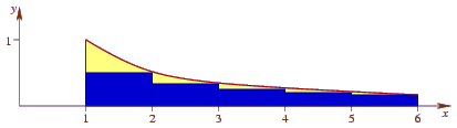
The rectangles represent the different terms of the sum: Each has a width of 1 and a height of 1/j for successive j. We want to find the area of the rectangles. To get an upper bound on the area, we draw the curve f(x) = 1/x between x = 1 and x = n, which is always above the rectangles. The area under the curve is ∫1n 1/x dx = [ln x]1n = ln n.
Substituting this for the total time executing Loop C, we have
The rest of the method takes O(n) time, so the overall the bound is O(n log n).
(We could have lost something in our estimate when we bounded the sum of primes' reciprocals by the sum of all reciprocals. In fact, there is an obscure mathematical fact that the sum of reciprocals of primes up to k is approximately (ln ln k) + 0.2614…. Using this fact, we get an even better bound of O(n log log n).)
4.4. Memory usage analysis
Although computer scientists don't talk about it nearly as often, big-O analysis can be applied to memory as well as time. For example, the prime-counting program of Figure 4.5 requires O(n / log n) memory, since it stores all the primes up to n in a list, and there are O(n / log n) such numbers.
Actually, this memory bound isn't technically correct. If n becomes really big, then we need to take into account the fact that the representation of the really big prime numbers don't actually take O(1) memory: A number k requires O(log k) memory to store k's digits. Thus, really, the amount of memory needed is O(n).
But if we were going to worry about that, then our time analysis should also take into account the fact that dividing two really big numbers doesn't take O(1) time either: The long division algorithm takes O(log² n) time. It simplifies things a lot — and for most real problems it doesn't really hurt us — if we just disregard these details and assume that each arithmetic operation take O(1) time, and storing each number takes O(1) space.
We can do better. Consider the algorithm of Figure 4.7.
Figure 4.7: A memory-free method for counting primes.
public static int memorylessCountPrimes(int n) {

    int count = 1;

    for(int k = 3; k <= n; k += 2) {

        if(testPrimality2(k)) count++;

    }

    return count;

}


private static boolean testPrimality2(int k) {

    if(k % 2 == 0) return k == 2;

    for(int i = 3; i * i <= k; i += 2) {

        if(k % i == 0) return false;

    }

    return true;

}
In this algorithm, we
don't store prime numbers in memory, and a result, we use only
O(1) memory. (Again, the real bound would be
O(log n) if
we were worrying about storing all the different digits of n.
But we're not worrying about that.)
This memory savings comes at the expense of a few more divisions,
because testPrimality2 can't restrict its tests to only
the primes as with the testPrimality code in
Figure 4.5.
However, dividing only by primes doesn't really save all that
much in terms of time: The Figure 4.5
algorithm takes roughly
O(n3/2 / (log n)²) time,
whereas the Figure 4.7 algorithm
takes O(n3/2) time. Our new algorithm
is moderately slower
than before, but it uses much less memory.
This is a general principle called the
Let's look at another example of the memory versus speed tradeoff. Consider the problem of stealing from a jewelry store, where we have a bag that can carry a certain amount of weight, and we want to select the most valuable subset of the jewelry in the store fitting into our bag.
One approach to this is to iterate through all the subsets of
the jewelry, using a recursive approach similar to the
printSubsets method of Section 2.1.
If we have n pieces of jewelry to choose from, there will be
2n subsets to consider, so that method will take
O(2n)
time. Since the method only remembers the current subset at any
instant as it progresses, it requires O(n) memory.
An alternative approach is to determine the best subset for each possible capacity, working ourselves up toward the bag's capacity, which we'll call C. We begin at 0, for which we can't carry any jewelry, a choice that has value 0. Then we progress to 1, where the best subset is the most valuable piece weighing 1 gram. Then we progress to 2, where the best subset is either the most valuable piece weighing 2 grams, or the best 1-gram subset, plus the most valuable 1-gram piece not in the best 1-gram subset. We can continue doing this.
In this alternative approach, we'll require O(C n) time: We go through C different capacities; for each capacity k, we consider each of the n pieces, seeing the value of including that piece (of weight w) in with the best subset weighing k − w grams, if that subset doesn't already contain the piece in question. This O(C n) bound is likely to be much better than O(2n); but it comes at the expense of memory: It requires O(C n) memory, whereas the all-subsets approach requires only O(n) memory.

Data & Procedure is licensed under a Creative Commons Attribution-Share Alike 3.0 License.
Based on a work at http://www.cburch.com/books/data/.